Cebranopadol (Kleideiter 2018) • nlmixr2lib

library(nlmixr2lib)
library(PKNCA)
#> 
#> Attaching package: 'PKNCA'
#> The following object is masked from 'package:stats':
#> 
#>     filter
library(rxode2)
#> rxode2 5.1.2 using 2 threads (see ?getRxThreads)
#>   no cache: create with `rxCreateCache()`
library(dplyr)
#> 
#> Attaching package: 'dplyr'
#> The following objects are masked from 'package:stats':
#> 
#>     filter, lag
#> The following objects are masked from 'package:base':
#> 
#>     intersect, setdiff, setequal, union
library(tidyr)
library(ggplot2)

Model and source

Citation: Kleideiter E, Piana C, Wang S, Nemeth R, Gautrois M. Clinical pharmacokinetic characteristics of cebranopadol, a novel first-in-class analgesic. Clin Pharmacokinet. 2018;57(1):31-50.
DOI: https://doi.org/10.1007/s40262-017-0545-1
Article: https://link.springer.com/article/10.1007/s40262-017-0545-1
Erratum: https://doi.org/10.1007/s40262-018-0686-x (Clin Pharmacokinet. 2018;57(11):1467-1469)

The erratum corrects Table 14 covariate-effect simulation results and several paragraphs of the Section 3 discussion. Where erratum-corrected values differ from the original article, the corrected values are the source of record for the model and this vignette.

Population

Kleideiter 2018 fits a two-compartment population PK model with two lagged transition compartments and first-order elimination to 14 pooled clinical trials of oral cebranopadol (a novel first-in-class NOP / opioid receptor agonist analgesic) in healthy adults and adult chronic-pain patients:

Phase I (8 trials, n = 287 pooled). Healthy adults receiving single oral doses of 0.8-800 ug or once-daily multiple doses up to 1600 ug. Three formulations (oral solution, film-coated tablet, liquid-filled capsule) were investigated and pooled in the population PK analysis (Table 12).
Phase IIa / II (6 trials, n = 1006 pooled). Adult patients with chronic pain across four indications: chronic low back pain (cLBP, two trials), osteoarthritis (OA) of the knee, painful diabetic polyneuropathy (DPN, three trials), and post-bunionectomy acute pain (one trial), each at multiple dose levels with 4-14 weeks of once-daily dosing.

The pooled analysis cohort is 1293 subjects (617 men and 676 women per the Discussion paragraph 4). Phase I subjects have median age 33 y (range 18-64) and phase II subjects have median age 58 y (range 18-79); pooled weight range is approximately 45-197 kg (Table 12 minimum to maximum across trials). Genotype-derived CYP2C9 phenotype is available for 38.3% of subjects; the remaining 61.7% are coded as unknown and form the model’s CYP2C9 reference category.

Reference covariate values (Kleideiter 2018 Table 14 footnote, erratum-corrected) used for the parameter-estimation typical-value computation:

sex = male (Table 14 simulation reference) / sex = female (Table 13 parameter-estimation reference: the most-common category)
formulation = tablet
CYP2C9 status = unknown
disease status = LBP and OA patients (nociceptive pain)
age = 55 years
CrCl = 106.4 mL/min
body weight = 82 kg
ALT = 19 U/L

Note that the Table 13 typical-value reference for sex (female) differs from the Table 14 simulation reference (male). The model file encodes parameters with female (SEXF = 1) as the reference and applies the +17.6% male-vs-female CL ratio via e_male_cl^(1 - SEXF); this matches the Table 13 typical-value column directly and reproduces the Table 14 sex effect after the simulation reference is switched.

Programmatic access to the population summary: readModelDb("Kleideiter_2018_cebranopadol")$population.

Source trace

The per-parameter origin is recorded as an in-file comment next to each ini() entry in inst/modeldb/specificDrugs/Kleideiter_2018_cebranopadol.R. The table below collects them in one place for review.

Equation / parameter	Value	Source location
`lcl` (CL/F, L/h)	log(74.3)	Kleideiter 2018 Table 13 Clearance Reference value
`lvc` (Vc/F, L)	log(225)	Kleideiter 2018 Table 13 Volume central compartment Reference value
`lvp` (Vp/F, L)	log(6750)	Kleideiter 2018 Table 13 Volume peripheral compartment Reference value
`lq` (Q/F, L/h)	log(84.2)	Kleideiter 2018 Table 13 Intercompartmental clearance
`lka` (Ka, 1/h)	log(0.864)	Kleideiter 2018 Table 13 Absorption rate constant Reference value
`lklag` (klag, 1/h)	log(0.087)	Kleideiter 2018 Table 13 klag Reference value
`e_male_cl`	1.176	Kleideiter 2018 Table 13 Male CL 87.4 / Female CL 74.3
`e_em_cl`	1.109	Kleideiter 2018 Table 13 CYP2C9 EM CL 82.4 / Reference CL 74.3
`e_pim_cl`	0.790	Kleideiter 2018 Table 13 CYP2C9 PIM CL 58.7 / Reference CL 74.3
`e_alt_cl`	-0.156	Kleideiter 2018 Table 13 Effect of ALT (exponential)
`e_crcl_cl`	0.349	Kleideiter 2018 Table 13 Effect of CrCl (exponential)
`e_age_vc`	-0.446	Kleideiter 2018 Table 13 Effect of age (exponential) on Vc
`e_wt_vp`	0.604	Kleideiter 2018 Table 13 Effect of body weight (exponential) on Vp
`e_solution_ka`	2.813	Kleideiter 2018 Table 13 Oral-solution Ka 2.43 / Reference Ka 0.864
`e_capsule_ka`	2.419	Kleideiter 2018 Table 13 Capsules Ka 2.09 / Reference Ka 0.864
`e_solution_klag`	0.885	Kleideiter 2018 Table 13 Oral-solution klag 0.077 / Reference klag 0.087
`e_capsule_klag`	0.885	Kleideiter 2018 Table 13 Capsules klag 0.077 / Reference klag 0.087
`e_solution_f`	1.045	Kleideiter 2018 Table 13 Bioavailability Oral solution
`e_capsule_f`	1.174	Kleideiter 2018 Table 13 Bioavailability Capsules
`e_healthy_f`	0.837	Kleideiter 2018 Table 13 Bioavailability Healthy volunteers
`e_bun_f`	1.801	Kleideiter 2018 Table 13 (erratum-corrected; original Table-13 row labeled ‘DPN patients’)
`e_dpn_f`	1.132	Kleideiter 2018 Table 13 (erratum-corrected; original Table-13 row labeled ‘Bunionectomy patients’)
IIV CL (omega^2)	0.412 (RSE 10.1%)	Kleideiter 2018 Table 13 IIV column
IIV Vc (omega^2)	0.559 (RSE 20.6%)	Kleideiter 2018 Table 13 IIV column
IIV Ka (omega^2)	0.519 (RSE 11.2%)	Kleideiter 2018 Table 13 IIV column
IIV klag (omega^2)	0.0626 (RSE 18.8%)	Kleideiter 2018 Table 13 IIV column
`propSd`	0.35 (approximated; see Assumptions)	Class-typical popPK value; Kleideiter 2018 does not report a residual-error magnitude in Table 13 or the Results narrative
Equations: 2-cmt + 2 transit + 1st-order elimination	n/a	Kleideiter 2018 Methods 2.4.1 + Results 3.2.7

Virtual cohort

The original observed dataset is not publicly available. This vignette constructs a typical-value simulation cohort matched to the Table 14 erratum reference scenario (male, tablet, CYP2C9 unknown, LBP / OA, age 55 y, CrCl 106.4 mL/min, weight 82 kg, ALT 19 U/L), plus the Table 14 covariate perturbation arms (female sex, lower CrCl, healthy / DPN / bunionectomy disease status), to reproduce the Table 14 erratum-corrected steady-state exposure metrics under the published 600 ug titration regimen.

set.seed(545L) # last 3 digits of original DOI 10.1007/s40262-017-0545-1

ref_covariates <- list(
  SEXF          = 0L,    # male = Table 14 simulation reference
  AGE           = 55,
  WT            = 82,
  CRCL          = 106.4,
  ALT           = 19,
  FORM_CAPSULE  = 0L,
  FORM_SOLUTION = 0L,
  CYP2C9_EM     = 0L,
  CYP2C9_PIM    = 0L,
  DIS_HEALTHY   = 0L,
  DIS_DPN       = 0L,
  DIS_BUNIONECTOMY = 0L
)

# One subject per arm, deterministic (zero between-subject variance) so the
# typical-value Cmax,ss and AUCss can be compared directly against Table 14
# erratum-corrected numbers.
make_arm <- function(arm_label, override = list(), id_offset = 0L) {
  cov <- modifyList(ref_covariates, override)
  data.frame(
    id            = id_offset + 1L,
    arm           = arm_label,
    SEXF          = cov$SEXF,
    AGE           = cov$AGE,
    WT            = cov$WT,
    CRCL          = cov$CRCL,
    ALT           = cov$ALT,
    FORM_CAPSULE  = cov$FORM_CAPSULE,
    FORM_SOLUTION = cov$FORM_SOLUTION,
    CYP2C9_EM     = cov$CYP2C9_EM,
    CYP2C9_PIM    = cov$CYP2C9_PIM,
    DIS_HEALTHY   = cov$DIS_HEALTHY,
    DIS_DPN       = cov$DIS_DPN,
    DIS_BUNIONECTOMY = cov$DIS_BUNIONECTOMY
  )
}

arms <- bind_rows(
  make_arm("Reference (male, LBP/OA)",  id_offset =  0L),
  make_arm("Female",                    list(SEXF = 1L),                id_offset =  1L),
  make_arm("Age 40 y",                  list(AGE = 40),                 id_offset =  2L),
  make_arm("Age 75 y",                  list(AGE = 75),                 id_offset =  3L),
  make_arm("CrCl 45 mL/min",            list(CRCL = 45),                id_offset =  4L),
  make_arm("CrCl 60 mL/min",            list(CRCL = 60),                id_offset =  5L),
  make_arm("CrCl 80 mL/min",            list(CRCL = 80),                id_offset =  6L),
  make_arm("WT 70 kg",                  list(WT = 70),                  id_offset =  7L),
  make_arm("WT 100 kg",                 list(WT = 100),                 id_offset =  8L),
  make_arm("WT 120 kg",                 list(WT = 120),                 id_offset =  9L),
  make_arm("Healthy",                   list(DIS_HEALTHY = 1L),         id_offset = 10L),
  make_arm("DPN",                       list(DIS_DPN = 1L),             id_offset = 11L),
  make_arm("Bunionectomy",              list(DIS_BUNIONECTOMY = 1L),    id_offset = 12L)
)
stopifnot(!anyDuplicated(arms$id))
n_arms <- nrow(arms)

Simulation

Each arm receives the published 600 ug titration regimen (100 ug x 6 days, 200 ug x 6 days, 400 ug x 6 days, then 600 ug q24h) for 40 days of total treatment, by which point the steady state is reached per the Table 14 erratum footnote (“the steady-state was defined to be achieved on Day 40”).

dose_schedule <- bind_rows(
  data.frame(day = 1:6,   amt = 100),
  data.frame(day = 7:12,  amt = 200),
  data.frame(day = 13:18, amt = 400),
  data.frame(day = 19:40, amt = 600)
)
dose_times <- (dose_schedule$day - 1) * 24

# Day 40 (last 24 h dosing interval) dense sampling for Cmax,ss and AUCss.
ss_dose_time   <- 39 * 24    # start of the day-40 dose
ss_obs_times   <- ss_dose_time + c(0, 0.5, 1, 2, 3, 4, 5, 6, 7, 8, 10, 12, 16, 20, 24)

# Trough sampling across the titration to show the approach to steady state.
trough_times   <- (seq(0, 40, by = 1)) * 24

all_obs_times  <- sort(unique(c(trough_times, ss_obs_times)))

# Replicate each arm row across dose events
dose_recs <- arms[rep(seq_len(n_arms), each = nrow(dose_schedule)), ] |>
  mutate(
    time = rep(dose_times,         times = n_arms),
    amt  = rep(dose_schedule$amt,  times = n_arms),
    evid = 1L,
    cmt  = "depot"
  )

obs_recs <- arms[rep(seq_len(n_arms), each = length(all_obs_times)), ] |>
  mutate(
    time = rep(all_obs_times, times = n_arms),
    amt  = 0,
    evid = 0L,
    cmt  = "central"
  )

events <- bind_rows(dose_recs, obs_recs) |>
  arrange(id, time, desc(evid)) |>
  select(id, time, amt, evid, cmt, arm,
         SEXF, AGE, WT, CRCL, ALT,
         FORM_CAPSULE, FORM_SOLUTION,
         CYP2C9_EM, CYP2C9_PIM,
         DIS_HEALTHY, DIS_DPN, DIS_BUNIONECTOMY)

stopifnot(!anyDuplicated(unique(events[, c("id", "time", "evid")])))

mod <- readModelDb("Kleideiter_2018_cebranopadol")
# Typical-value (zero between-subject variance) simulation so the simulated
# Cmax,ss and AUCss can be compared head-to-head against the Table 14 erratum
# typical-patient predictions.
mod_typical <- rxode2::zeroRe(mod)
#> ℹ parameter labels from comments will be replaced by 'label()'
sim <- rxode2::rxSolve(mod_typical, events = events, keep = c("arm")) |>
  as.data.frame()
#> ℹ omega/sigma items treated as zero: 'etalcl', 'etalvc', 'etalka', 'etalklag'
#> Warning: multi-subject simulation without without 'omega'

Approach to steady state during the 600 ug titration

trough_sim <- sim |>
  filter(time %in% trough_times) |>
  mutate(day = time / 24)

ggplot(
  trough_sim |> filter(arm == "Reference (male, LBP/OA)"),
  aes(day, Cc)
) +
  geom_line(linewidth = 0.8, colour = "steelblue") +
  geom_vline(xintercept = c(6, 12, 18), linetype = "dashed", colour = "grey60") +
  annotate("text", x = c(3, 9, 15, 30), y = max(trough_sim$Cc) * 0.9,
           label = c("100 ug", "200 ug", "400 ug", "600 ug"), size = 3) +
  labs(
    x       = "Day after first dose",
    y       = "Trough cebranopadol concentration (pg/mL)",
    title   = "Typical-value trough profile during the 600 ug titration",
    caption = "Reference covariate set: male, tablet, CYP2C9 unknown, LBP/OA, age 55 y, CrCl 106.4 mL/min, WT 82 kg, ALT 19 U/L."
  ) +
  theme_bw()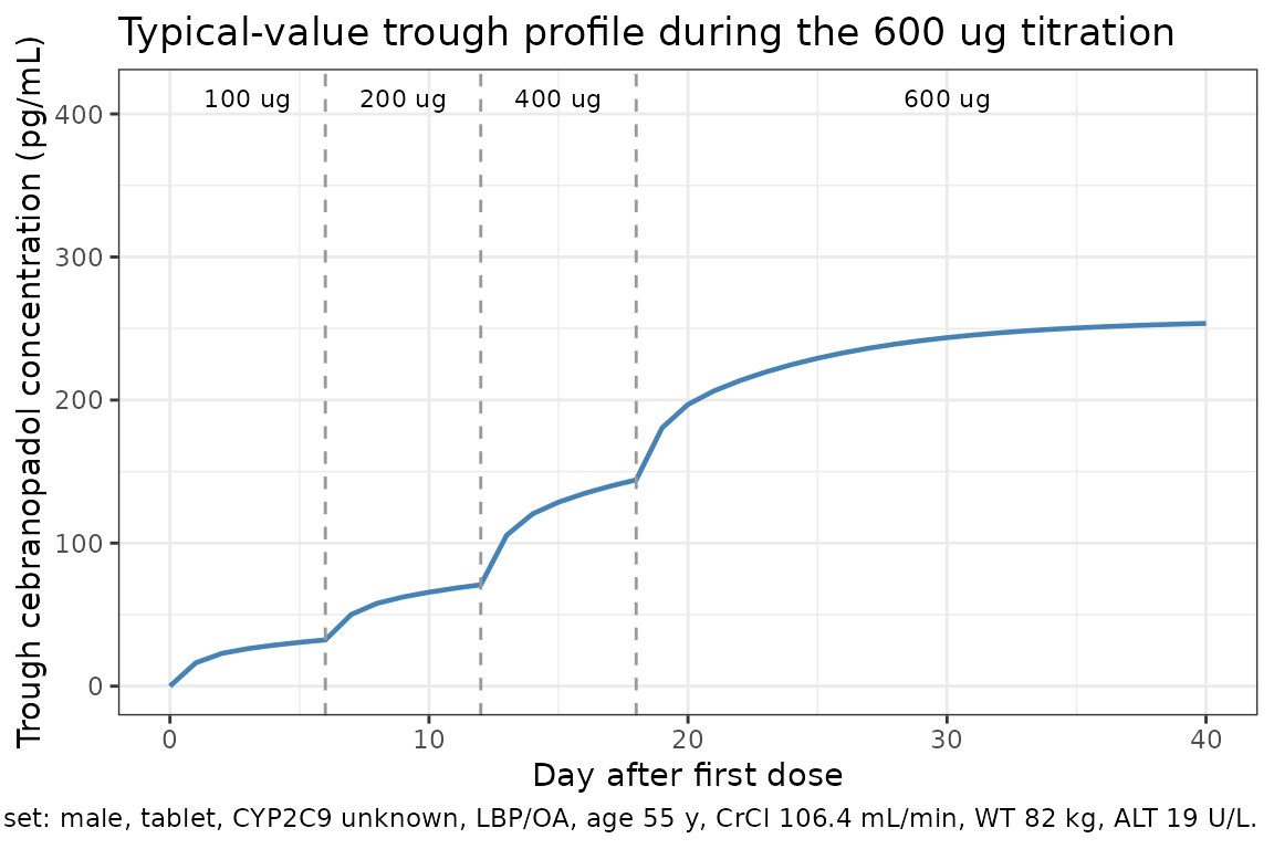

Replicate Kleideiter 2018 Table 14 (erratum-corrected) covariate effects

Table 14 (erratum) tabulates typical-patient Cmax,ss and AUCss values under the 600 ug titration regimen for each covariate-perturbation arm, expressed as % change relative to the reference patient.

# Day 40 (last 24-h interval) dense observations, time shifted so each arm has
# a t = 0 at the start of the day-40 dose.
ss_block <- sim |>
  filter(time %in% ss_obs_times) |>
  mutate(time = time - ss_dose_time) |>
  select(id, time, Cc, arm)

# Dose record at t = 0 of the shifted interval (600 ug on the steady-state day).
dose_block <- ss_block |>
  group_by(id) |>
  summarise(time = 0, amt = 600, arm = first(arm), .groups = "drop")

conc_obj <- PKNCA::PKNCAconc(
  ss_block,
  Cc ~ time | arm + id,
  concu = "pg/mL", timeu = "hr"
)
dose_obj <- PKNCA::PKNCAdose(
  dose_block,
  amt ~ time | arm + id,
  doseu = "ug"
)

intervals <- data.frame(
  start    = 0,
  end      = 24,
  cmax     = TRUE,
  auclast  = TRUE
)

nca_res <- PKNCA::pk.nca(PKNCA::PKNCAdata(conc_obj, dose_obj, intervals = intervals))

table14_sim <- as.data.frame(nca_res$result) |>
  filter(PPTESTCD %in% c("cmax", "auclast")) |>
  select(arm, PPTESTCD, PPORRES) |>
  pivot_wider(names_from = PPTESTCD, values_from = PPORRES) |>
  rename(Cmax_ss_sim = cmax, AUC_ss_sim = auclast)

ref_row <- table14_sim |> filter(arm == "Reference (male, LBP/OA)")
ref_cmax <- ref_row$Cmax_ss_sim
ref_auc  <- ref_row$AUC_ss_sim

table14_sim <- table14_sim |>
  mutate(
    Cmax_pct_sim = 100 * (Cmax_ss_sim - ref_cmax) / ref_cmax,
    AUC_pct_sim  = 100 * (AUC_ss_sim  - ref_auc ) / ref_auc
  )

# Published Table 14 erratum values (Cmax,ss in pg/mL, AUCss in pg*h/mL, percent
# change relative to the male reference patient).
table14_pub <- tibble::tribble(
  ~arm,                       ~Cmax_ss_pub, ~Cmax_pct_pub, ~AUC_ss_pub, ~AUC_pct_pub,
  "Reference (male, LBP/OA)",        378,          0,           6790,         0,
  "Female",                          432,         14,           7960,        17,
  "Age 40 y",                        375,         -1,           6790,         0,
  "Age 75 y",                        381,          1,           6790,         0,
  "CrCl 45 mL/min",                  483,         28,           9080,        34,
  "CrCl 60 mL/min",                  446,         18,           8250,        21,
  "CrCl 80 mL/min",                  410,          9,           7480,        10,
  "WT 70 kg",                        379,          0,           6810,         0,
  "WT 100 kg",                       377,          0,           6760,        -1,
  "WT 120 kg",                       375,         -1,           6720,        -1,
  "Healthy",                         316,        -16,           5690,       -16,
  "DPN",                             428,         13,           7690,        13,
  "Bunionectomy",                    681,         80,          12200,        80
)

table14_compare <- table14_pub |>
  left_join(table14_sim, by = "arm") |>
  select(arm,
         Cmax_ss_pub, Cmax_ss_sim, Cmax_pct_pub, Cmax_pct_sim,
         AUC_ss_pub,  AUC_ss_sim,  AUC_pct_pub,  AUC_pct_sim)

knitr::kable(
  table14_compare,
  digits  = c(0, 0, 0, 0, 1, 0, 0, 0, 1),
  caption = paste(
    "Simulated typical-value Cmax,ss (pg/mL) and AUCss (pg*h/mL) under the",
    "600 ug titration regimen vs Kleideiter 2018 Table 14 erratum-corrected",
    "published values. Percent changes are relative to the reference patient."
  )
)

Simulated typical-value Cmax,ss (pg/mL) and AUCss (pg*h/mL) under the 600 ug titration regimen vs Kleideiter 2018 Table 14 erratum-corrected published values. Percent changes are relative to the reference patient.
arm	Cmax_ss_pub	Cmax_ss_sim	Cmax_pct_pub	Cmax_pct_sim	AUC_ss_pub	AUC_ss_sim	AUC_pct_pub	AUC_pct_sim
Reference (male, LBP/OA)	378	306	0	0.0	6790	6786	0	0.0
Female	432	356	14	16.3	7960	7943	17	17.0
Age 40 y	375	306	-1	-0.1	6790	6785	0	0.0
Age 75 y	381	306	1	0.2	6790	6786	0	0.0
CrCl 45 mL/min	483	404	28	32.2	9080	9069	34	33.7
CrCl 60 mL/min	446	369	18	20.5	8250	8237	21	21.4
CrCl 80 mL/min	410	336	9	9.7	7480	7476	10	10.2
WT 70 kg	379	307	0	0.3	6810	6807	0	0.3
WT 100 kg	377	304	0	-0.5	6760	6750	-1	-0.5
WT 120 kg	375	303	-1	-1.1	6720	6707	-1	-1.2
Healthy	316	256	-16	-16.3	5690	5680	-16	-16.3
DPN	428	346	13	13.2	7690	7681	13	13.2
Bunionectomy	681	551	80	80.1	12200	12221	80	80.1

The simulated percent-change column should reproduce the Table 14 erratum percent-change column closely for the categorical covariate arms (sex, disease status); the absolute Cmax,ss and AUCss values may differ from the published numbers because the structural interpretation of the transit- compartment absorption chain affects the entire concentration-time profile shape. See Assumptions and deviations for details.

Assumptions and deviations

Transit-compartment structural interpretation. Kleideiter 2018 Section 3.2.7 describes the absorption model as “a two-compartment disposition model with two lagged transition compartments” without writing out the explicit ODEs, and Table 13 reports two formulation-dependent rate constants Ka and klag whose individual roles in the chain are not stated. The model file uses the biologically-motivated reading in which Ka governs the depot-to- transit1 step (dissolution-limited absorption from the dosage form; values vary ~2.8-fold across tablet, capsule, and oral solution) and klag governs both subsequent transit steps (transit1 -> transit2 -> central; uniform 0.077- 0.087 1/h across formulations). The alternative reading - klag at the depot + transit1 steps and Ka at the final transit2 -> central step (the Bienczak 2016 nevirapine convention used elsewhere in nlmixr2lib) - is equally consistent with the paper’s prose; without the NONMEM control stream or appendix, the ambiguity cannot be resolved from on-disk sources. Either reading places the rate-limiting step at the slow klag rate, so the simulated peak time and concentration-time-profile shape will not precisely reproduce the paper’s reported Tmax of 4-6 h (the NCA-derived Tmax from the single-dose trials). The Table 14 covariate-percent-change comparison is more robust to this structural ambiguity than the absolute Cmax,ss / AUCss numbers because percent changes within an arm cancel the common transit-time scale.
Residual-error magnitude. Kleideiter 2018 Section 2.4.1 specifies the residual-error model as additive on log-transformed cebranopadol concentrations (equivalent to proportional residual error on the linear scale in the nlmixr2 idiom), but Table 13 and the Results narrative do not report the residual-error variance estimate. The model file uses a class-typical approximation propSd = 0.35 (about 35% proportional CV on the linear scale, a representative value for orally-dosed small-molecule analgesics with mixed intensive + sparse-sampling popPK datasets). This value affects the width of stochastic VPCs (irrelevant for the deterministic Table 14 reproduction above) but not the typical- value Cmax,ss / AUCss predictions.
Sex reference category divergence between Table 13 and Table 14. The Table 13 parameter-estimation reference uses female sex (the most-common category in the analysis cohort), while the Table 14 simulation reference uses male sex (the typical-patient simulation choice). The model file preserves the Table 13 reference - female corresponds to SEXF = 1, the typical-value CL is 74.3 L/h, and male is encoded as the +17.6% multiplier applied via e_male_cl^(1 - SEXF). This vignette’s reference-arm simulation switches to the Table 14 male reference for side-by-side comparison.
CYP2C9 unknown-phenotype reference. Only 38.3% of the analysis cohort had a known CYP2C9 phenotype; the remaining 61.7% are coded as unknown and form the model’s CYP2C9 reference category. The canonical CYP2C9_EM covariate’s standard reference (in Jeong 2022) is IM/PM only, not unknown. In the Kleideiter 2018 model, the 0-level of CYP2C9_EM pools unknown + non-EM phenotypes, and a sibling new canonical CYP2C9_PIM carries the PIM-vs-unknown contrast. Both indicators are 0 for the reference-arm simulations above.
Four-level disease-state encoding via three indicators. The model encodes the four-category disease factor (LBP and OA reference + healthy, DPN, bunionectomy) using three binary indicators DIS_HEALTHY, DIS_DPN, and DIS_BUNIONECTOMY, two of which (DIS_DPN, DIS_BUNIONECTOMY) are registered as new canonical covariates alongside this model. When all three are 0 the subject is in the LBP / OA reference category (the Table 13 most-common-category reference).
Three-level formulation encoding via two indicators. The model encodes the three-category formulation factor (tablet reference + oral solution + liquid-filled capsule) using two binary indicators FORM_SOLUTION (new canonical registered alongside this model) and FORM_CAPSULE (existing canonical, reused with the tablet reference documented per-model). When both are 0 the subject is in the tablet reference category.
Food and CYP2D6 effects not retained. Kleideiter 2018 Methods Section 2.4.1 tested food intake on the absorption rate constant and CYP2D6 phenotype on CL during covariate selection; neither was retained in the final model (Results 3.2.7 paragraphs 5-7). The model file therefore does not include FED or CYP2D6_* covariates. Future cebranopadol simulations that require a food-effect term should consult the paper’s Section 3.2.6 single-dose ANOVA estimates (mean Cmax and AUCt ~30% higher under fed vs fasted conditions) rather than the population PK model.
Erratum supersedes original Table 14. The Cmax,ss / AUCss percent- change values in the published-vs-simulated comparison above are taken from the 2018 erratum’s revised Table 14, not the original 2018 article Table 14, per the Phase 1 step 8 errata-handling convention.