Busulfan (Protzenko 2025)
Source:vignettes/articles/Protzenko_2025_busulfan.Rmd
Protzenko_2025_busulfan.RmdModel and source
- Citation: Protzenko D, Bouchacourt B, Carriat L, Maroselli P, Boeri C, Devillier R, Ciccolini J. Adaptive dosing of high-dose busulfan in real-world adult patients undergoing haematopoietic cell transplant conditioning. Br J Clin Pharmacol. 2025;91(4):1171. doi:10.1111/bcp.16343
- Description: One-compartment IV-infusion population PK prior for high-dose once-daily busulfan in adults undergoing haematopoietic cell transplant conditioning, parameterised on the inverse volume of distribution (1/V) and the elimination rate constant k with correlated additive-normal between-subject variability, from a standard two-stage analysis of 16 richly sampled patients and used as the Bayesian prior for three-sample adaptive dosing (Protzenko 2025)
- Article: https://doi.org/10.1111/bcp.16343
Protzenko 2025 describes a real-world programme of Bayesian adaptive dosing for high-dose, once-daily intravenous busulfan in adults conditioned for haematopoietic cell transplantation. The pharmacokinetic engine is a one-compartment model with a 3-h zero-order infusion. Its population prior was built by the standard two-stage method from 16 richly sampled patients: each profile was fitted individually by weighted least squares, and the mean vector and covariance matrix of the individual estimates became the prior.
Two features of the prior determine how the packaged model is written:
-
The estimated parameters are
1/Vandk, notCLandV. Clearance is derived,CL = V * k. -
The between-subject distribution is Gaussian on that linear
scale (“assuming Gaussian distribution for interindividual
variability”). The random effects are therefore additive on
1/Vand onk, and they are correlated, rather than exponential onVandCL.
Population
The prior comes from 16 adults undergoing haematopoietic cell transplantation with high-dose busulfan in the HGB-207 protocol (EudraCT 2015-004122-33), each with eight samples from 2 to 12 h after the start of the infusion. The paper does not report their demographics.
The prior was then applied to 71 adults treated between January 2016 and September 2022 at the Institut Paoli Calmettes, Marseille (Table 1): age 53 +/- 14 years (range 19-71), 49% female, weight 73 +/- 17 kg (range 40-135), body surface area 1.87 +/- 0.26 m^2. The commonest diagnoses were acute myeloid leukaemia (31%), acute lymphoblastic leukaemia (21%) and myelofibrosis (14%). Every patient received fludarabine. Busulfan was started at 3 mg/kg once daily as a 3-h infusion, for four doses (n = 60), five (n = 5) or six (n = 6), with a cumulative AUC target of 66.0 mg*h/L (42% of patients), 82.6 mg*h/L (17%) or 87.6 mg*h/L (39%). Three samples taken after the first dose, at 3 h 15 min, 9 h and 12 h after the start of the infusion, gave the individual Bayesian estimates used to adjust the remaining doses.
The same information is available programmatically via
readModelDb("Protzenko_2025_busulfan")()$population.
Source trace
| Equation / parameter | Value | Source location |
|---|---|---|
lvc |
log(1 / 2.277e-2), V = 43.92 L |
Methods, mean population parameters:
1/V = 2.277e-2 L^-1
|
lkel |
log(0.2448) |
Methods, mean population parameters:
k = 2.448e-1 h^-1
|
etavcinv |
2.018e-5 L^-2 | Methods, covariance matrix, element (1,1) |
etavcinv-etakel covariance |
3.104e-5 L^-1 h^-1 | Methods, covariance matrix, elements (1,2) and (2,1) |
etakel |
5.338e-4 h^-2 | Methods, covariance matrix, element (2,2) |
propSd |
0 (held) | Methods: proportional error variance in the first-stage fits; magnitude not reported |
| One-compartment infusion model | n/a | Methods, the two printed expressions for c(t) during
and after the infusion |
CL = V * k, AUC = D / CL,
t1/2 = ln 2 / k
|
n/a | Methods, derived individual parameters |
Adapted dose D* = (AUC* - AUC_i) * CL_i / n
|
n/a | Methods, adaptive-dosing equation (n = remaining
administrations) |
Typical values and the printed closed form
The typical values follow directly from the mean vector. The model must also reproduce the paper’s two closed-form expressions for the concentration during and after a zero-order infusion,
-
c(t) = D/T * 1/(kV) * (1 - exp(-k t))for0 <= t < T, and -
c(t) = D/T * 1/(kV) * (exp(-k (t - T)) - exp(-k t))fort >= T.
Both sides of this check use the same parameters, so the difference is pure numerical error and the bound is tight.
mod <- rxode2::rxode2(readModelDb("Protzenko_2025_busulfan"))
#> ℹ parameter labels from comments will be replaced by 'label()'
mod_typ <- rxode2::zeroRe(mod)

dose_typ <- 3 * 73 # 3 mg/kg at the cohort mean weight of 73 kg
t_inf <- 3
obs_t <- sort(unique(c(seq(0, 24, by = 0.25), 3.25, 9, 12)))

ev_typ <- rxode2::et(amt = dose_typ, dur = t_inf, cmt = "central") |>
  rxode2::et(obs_t, cmt = "central")
sim_typ <- rxode2::rxSolve(mod_typ, ev_typ, returnType = "data.frame")
#> ℹ omega/sigma items treated as zero: 'etavcinv', 'etakel'

v_typ <- 1 / 2.277e-2
k_typ <- 0.2448
closed_form <- function(t, d, tinf, k, v) {
  ifelse(
    t < tinf,
    d / tinf / (k * v) * (1 - exp(-k * t)),
    d / tinf / (k * v) * (exp(-k * (t - tinf)) - exp(-k * t))
  )
}
cf <- closed_form(sim_typ$time, dose_typ, t_inf, k_typ, v_typ)

tibble::tibble(
  Quantity = c("V (L)", "k (1/h)", "CL = V * k (L/h)", "t1/2 = ln 2 / k (h)"),
  Model = c(sim_typ$vc[1], sim_typ$kel[1], sim_typ$cl[1], log(2) / sim_typ$kel[1]),
  `From the mean vector` = c(v_typ, k_typ, v_typ * k_typ, log(2) / k_typ)
) |>
  dplyr::mutate(dplyr::across(-Quantity, \(x) signif(x, 4))) |>
knitr::kable(caption = "Typical values of the packaged model.")| Quantity | Model | From the mean vector |
|---|---|---|
| V (L) | 43.9200 | 43.9200 |
| k (1/h) | 0.2448 | 0.2448 |
| CL = V * k (L/h) | 10.7500 | 10.7500 |
| t1/2 = ln 2 / k (h) | 2.8310 | 2.8310 |
stopifnot(
  abs(sim_typ$cl[1] / (v_typ * k_typ) - 1) < 1e-8,
  max(abs(sim_typ$Cc - cf)) < 1e-4 * max(cf)
)
ggplot(sim_typ, aes(time, Cc)) +
  geom_line() +
  geom_point(data = tibble::tibble(time = obs_t, cf = closed_form(obs_t, dose_typ, t_inf, k_typ, v_typ)) |>
               dplyr::filter(time %in% c(3.25, 9, 12)),
             aes(time, cf), colour = "firebrick", size = 2.5) +
  labs(x = "Time after the start of the infusion (h)",
       y = "Busulfan concentration (mg/L)",
       title = "Typical profile after a 219 mg (3 mg/kg) 3-h infusion",
       caption = "Red points: the closed form at the three Bayesian sampling times (3.25, 9 and 12 h).")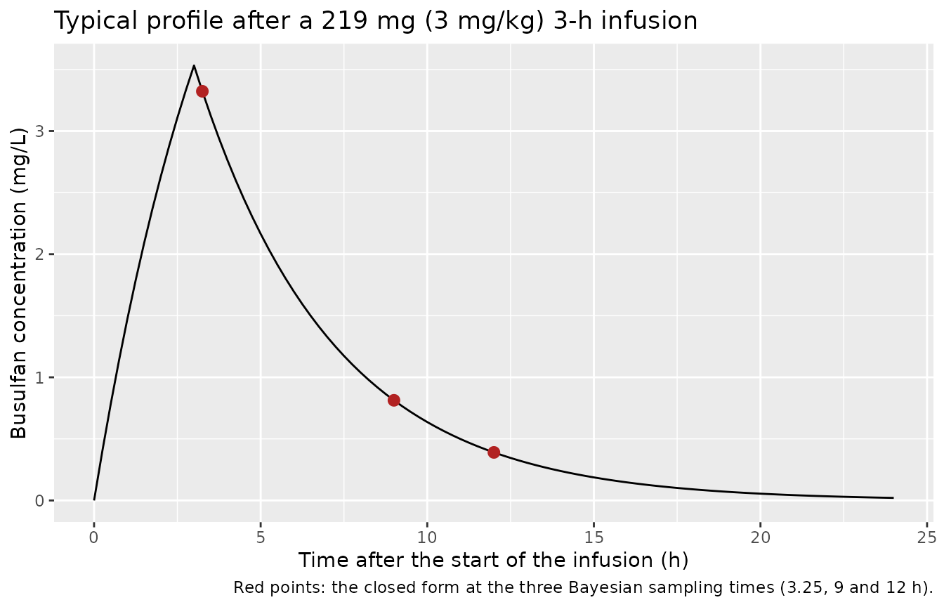
Between-subject variability
set.seed(20250414)

# Arms follow the Table 1 split of cumulative AUC targets (16 000, 20 000 and
# 21 200 uM*min); the single patient with an 18 000 uM*min target is folded
# into the 20 000 arm. Values in mg*h/L are those the paper prints.
arms <- tibble::tibble(
  target = c("66.0 mg*h/L", "82.6 mg*h/L", "87.6 mg*h/L"),
  auc_target = c(66.0, 82.6, 87.6),
  n = c(85L, 35L, 80L)
)

# Weight: log-normal matched to Table 1 (mean 73 kg, SD 17 kg), truncated to the
# observed 40-135 kg range.
subjects <- arms |>
  tidyr::uncount(n) |>
  dplyr::mutate(
    id = dplyr::row_number(),
    WT = pmin(pmax(73 * exp(stats::rnorm(dplyr::n(), -0.026, 0.23)), 40), 135),
    dose1 = 3 * WT
  )

ev1 <- dplyr::bind_rows(
  subjects |> dplyr::transmute(id, time = 0, amt = dose1, dur = t_inf,
                               evid = 1L, cmt = "central", target),
  subjects |> dplyr::select(id, target) |>
    tidyr::expand_grid(time = sort(unique(c(seq(0, 12, by = 0.25), seq(13, 48, by = 1))))) |>
    dplyr::mutate(amt = NA_real_, dur = NA_real_, evid = 0L, cmt = "central")
) |>
  dplyr::arrange(id, time, dplyr::desc(evid))

# Random effects are drawn once, in base R, from the model's covariance matrix
# and passed to every solve. The first-dose and the full-course simulations
# then describe the same patients, and the cohort does not depend on rxode2's
# random-number stream.
omega <- mod$omega
eta <- matrix(stats::rnorm(nrow(subjects) * nrow(omega)), nrow(subjects)) %*% chol(omega)
colnames(eta) <- rownames(omega)
eta_params <- data.frame(id = subjects$id, eta)

sim1 <- rxode2::rxSolve(mod_typ, ev1, params = eta_params, keep = "target",
                        returnType = "data.frame")
#> Warning: multi-subject simulation without without 'omega'
stopifnot(dplyr::n_distinct(sim1$id) == nrow(subjects))

indiv <- sim1 |>
  dplyr::group_by(id, target) |>
  dplyr::summarise(vcinv = vcinv[1], kel = kel[1], vc = vc[1], cl = cl[1],
                   .groups = "drop")

tibble::tibble(
  Quantity = c("Mean of 1/V (L^-1)", "SD of 1/V (L^-1)", "Mean of k (1/h)",
               "SD of k (1/h)", "Correlation of 1/V and k"),
  Simulated = c(mean(indiv$vcinv), sd(indiv$vcinv), mean(indiv$kel),
                sd(indiv$kel), stats::cor(indiv$vcinv, indiv$kel)),
  Prior = c(2.277e-2, sqrt(2.018e-5), 0.2448, sqrt(5.338e-4),
            3.104e-5 / sqrt(2.018e-5 * 5.338e-4))
) |>
  dplyr::mutate(dplyr::across(-Quantity, \(x) signif(x, 3))) |>
  knitr::kable(caption = paste(
    "Simulated individual parameters against the two-stage prior. The prior",
    "implies coefficients of variation of 19.7% on 1/V and 9.4% on k, with a",
    "correlation of 0.30."
))| Quantity | Simulated | Prior |
|---|---|---|
| Mean of 1/V (L^-1) | 0.02260 | 0.02280 |
| SD of 1/V (L^-1) | 0.00449 | 0.00449 |
| Mean of k (1/h) | 0.24600 | 0.24500 |
| SD of k (1/h) | 0.02260 | 0.02310 |
| Correlation of 1/V and k | 0.26500 | 0.29900 |
stopifnot(
  abs(stats::median(indiv$kel) / 0.2448 - 1) < 0.05,
  abs(stats::median(indiv$vcinv) / 2.277e-2 - 1) < 0.05
)
Clearance against the 71-patient Bayesian estimates
The paper reports the individual Bayesian clearances after the first dose in the 71-patient cohort as 12.0 +/- 3.1 L/h, with quartiles 9.8 and 13.9 L/h (Results, intra-patient variability; Figure 4). These are posterior estimates in a different cohort from the 16 patients behind the prior, so they are a consistency check on the prior’s location and spread, not a reproduction.
tibble::tibble(
  Statistic = c("Mean (L/h)", "SD (L/h)", "Q1 (L/h)", "Q3 (L/h)"),
  `Simulated from the prior` = c(mean(indiv$cl), sd(indiv$cl),
                                 stats::quantile(indiv$cl, 0.25),
                                 stats::quantile(indiv$cl, 0.75)),
  `Published, first dose` = c(12.0, 3.1, 9.8, 13.9)
) |>
  dplyr::mutate(`Simulated from the prior` = round(`Simulated from the prior`, 1)) |>
knitr::kable(caption = "Busulfan clearance: prior predictive versus the published first-dose Bayesian estimates.")| Statistic | Simulated from the prior | Published, first dose |
|---|---|---|
| Mean (L/h) | 11.3 | 12.0 |
| SD (L/h) | 2.4 | 3.1 |
| Q1 (L/h) | 9.6 | 9.8 |
| Q3 (L/h) | 12.6 | 13.9 |
# The prior's centre sits a little below the application cohort; a mis-scaled
# 1/V or k would move it by far more than this bound.
stopifnot(abs(stats::median(indiv$cl) / 12.0 - 1) < 0.2)
The prior predicts a typical clearance of 10.8 L/h and a coefficient of variation of roughly 20%, against 12.0 L/h and 26% in the application cohort. The narrower prior spread is expected: it reflects 16 selected trial patients, while the real-world cohort spans 40-135 kg and every patient in it is included without censoring.
sim1 |>
  dplyr::filter(time <= 24) |>
  dplyr::group_by(time) |>
  dplyr::summarise(Q05 = stats::quantile(Cc, 0.05), Q50 = stats::median(Cc),
                   Q95 = stats::quantile(Cc, 0.95), .groups = "drop") |>
  ggplot(aes(time, Q50)) +
  geom_ribbon(aes(ymin = Q05, ymax = Q95), alpha = 0.25) +
  geom_line() +
  geom_vline(xintercept = c(3.25, 9, 12), linetype = "dotted") +
  labs(x = "Time after the start of the first infusion (h)",
       y = "Busulfan concentration (mg/L)",
       title = "First-dose profiles after 3 mg/kg",
       caption = "Median and 5th-95th percentiles. Dotted lines: the three Bayesian sampling times.")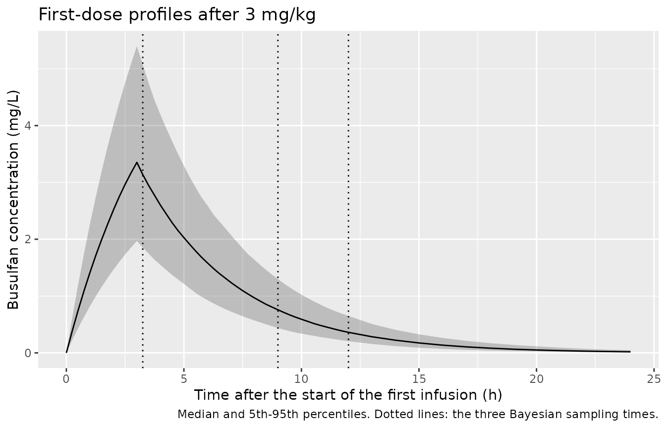
PKNCA validation of the first dose
nca1_conc <- sim1 |>
  dplyr::filter(!is.na(Cc)) |>
  dplyr::select(id, time, Cc, target)
nca1_conc <- dplyr::bind_rows(
  nca1_conc,
  nca1_conc |> dplyr::distinct(id, target) |> dplyr::mutate(time = 0, Cc = 0)
) |>
  dplyr::distinct(id, target, time, .keep_all = TRUE) |>
  dplyr::arrange(id, time)

nca1_dose <- subjects |> dplyr::transmute(id, target, time = 0, amt = dose1)

nca1 <- PKNCA::pk.nca(PKNCA::PKNCAdata(
  PKNCA::PKNCAconc(nca1_conc, Cc ~ time | target + id, concu = "mg/L", timeu = "h"),
  PKNCA::PKNCAdose(nca1_dose, amt ~ time | target + id, doseu = "mg"),
  intervals = data.frame(start = 0, end = Inf, cmax = TRUE, tmax = TRUE,
                         aucinf.obs = TRUE, half.life = TRUE, cl.obs = TRUE)
))
nca1_df <- as.data.frame(nca1)

nca1_wide <- nca1_df |>
  dplyr::filter(PPTESTCD %in% c("aucinf.obs", "cl.obs", "half.life", "cmax")) |>
  dplyr::select(id, target, PPTESTCD, PPORRES) |>
  tidyr::pivot_wider(names_from = PPTESTCD, values_from = PPORRES) |>
  dplyr::left_join(indiv |> dplyr::select(id, cl, kel), by = "id")

# NCA clearance and half-life against each subject's own model parameters.
stopifnot(
  abs(stats::median(nca1_wide$cl.obs / nca1_wide$cl) - 1) < 0.01,
  abs(stats::median(nca1_wide$half.life / (log(2) / nca1_wide$kel)) - 1) < 0.02
)

sim_summary <- nca1_wide |>
  dplyr::summarise(cl.obs = mean(cl.obs), half.life = mean(half.life))
reference <- tibble::tibble(cl.obs = 12.0, half.life = log(2) / 0.2448)

nlmixr2lib::ncaComparisonTable(
  simulated = sim_summary,
  reference = reference,
  params = c("cl.obs", "half.life"),
  units = c(cl.obs = "L/h", half.life = "h"),
  tolerance_pct = 20
) |>
  # Busulfan is given intravenously, so the observed clearance is CL, not CL/F.
  dplyr::mutate(`NCA parameter` = sub("CL/F", "CL", `NCA parameter`, fixed = TRUE)) |>
  knitr::kable(caption = paste(
    "First-dose NCA (cohort means) against the published mean first-dose",
    "Bayesian clearance (12.0 L/h) and the half-life implied by the prior mean",
    "k (ln 2 / 0.2448 h^-1). * marks a >20% difference."
))| NCA parameter | Reference | Simulated | % diff |
|---|---|---|---|
| t½ (h) | 2.83 | 2.84 | +0.2% |
| CL (L/h) | 12 | 11.3 | -5.7% |
Bayesian adaptive dosing (Figures 1 and 2)
The paper’s adjustment sets each remaining dose to
D* = (AUC* - AUC_1) * CL_i / n, where AUC* is
the cumulative target, AUC_1 the first-dose exposure and
n the number of remaining administrations. The simulation
below reproduces the four-dose regimen given to 60 of the 71 patients
(D-6, D-5, D-4 and D-2, so doses at 0, 24, 48 and 96 h). The first dose
is 3 mg/kg; AUC_1 and CL_i are taken from the
first-dose NCA above, which stands in for a Bayesian estimate with no
estimation error.
intermediate <- nca1_wide |>
  dplyr::left_join(subjects |> dplyr::select(id, auc_target, dose1), by = "id") |>
  dplyr::mutate(
    dev1 = 100 * (aucinf.obs / (auc_target / 4) - 1),
    dose_adj = (auc_target - aucinf.obs) * cl.obs / 3
  )

dose_times <- c(0, 24, 48, 96)
ev_course <- dplyr::bind_rows(
  intermediate |>
    dplyr::select(id, target, dose1, dose_adj) |>
    tidyr::expand_grid(dose_no = 1:4) |>
    dplyr::transmute(id, target, time = dose_times[dose_no],
                     amt = ifelse(dose_no == 1, dose1, dose_adj),
                     dur = t_inf, evid = 1L, cmt = "central"),
  intermediate |>
    dplyr::select(id, target) |>
    tidyr::expand_grid(time = seq(0, 144, by = 0.25)) |>
    dplyr::mutate(amt = NA_real_, dur = NA_real_, evid = 0L, cmt = "central")
) |>
  dplyr::arrange(id, time, dplyr::desc(evid))

sim_course <- rxode2::rxSolve(mod_typ, ev_course, params = eta_params,
                              keep = "target", returnType = "data.frame")
#> Warning: multi-subject simulation without without 'omega'

course_conc <- sim_course |>
  dplyr::filter(!is.na(Cc)) |>
  dplyr::select(id, time, Cc, target)
course_dose <- ev_course |>
  dplyr::filter(evid == 1) |>
  dplyr::select(id, target, time, amt)

nca_course <- PKNCA::pk.nca(PKNCA::PKNCAdata(
  PKNCA::PKNCAconc(course_conc, Cc ~ time | target + id, concu = "mg/L", timeu = "h"),
  PKNCA::PKNCAdose(course_dose, amt ~ time | target + id, doseu = "mg"),
  intervals = data.frame(start = c(0, 24, 48, 96), end = c(24, 48, 96, 144),
                         auclast = TRUE)
))

cumulative <- as.data.frame(nca_course) |>
  dplyr::filter(PPTESTCD == "auclast") |>
  dplyr::group_by(id, target) |>
  dplyr::summarise(cauc = sum(PPORRES), .groups = "drop") |>
  dplyr::left_join(intermediate |> dplyr::select(id, auc_target, dev1), by = "id") |>
  dplyr::mutate(dev_final = 100 * (cauc / auc_target - 1))

# With CL_i known exactly the adjustment is exact; the tolerance only covers
# trapezoidal error and the sub-0.1% tail beyond 144 h.
stopifnot(max(abs(cumulative$dev_final)) < 1)
summ_dev <- function(x) {
  c(`Mean absolute deviation (%)` = mean(abs(x)),
    `Q1 of absolute deviation (%)` = unname(stats::quantile(abs(x), 0.25)),
    `Q3 of absolute deviation (%)` = unname(stats::quantile(abs(x), 0.75)),
    `Outside +/-25% (%)` = 100 * mean(abs(x) > 25),
    `Minimum deviation (%)` = min(x),
    `Maximum deviation (%)` = max(x))
}

tibble::tibble(
  Statistic = names(summ_dev(cumulative$dev1)),
  `Simulated, standard dose` = round(summ_dev(cumulative$dev1), 1),
  `Published, standard dose` = c(19.5, 8.3, 27.3, 31, -47.6, 60.1),
  `Simulated, after adjustment` = round(summ_dev(cumulative$dev_final), 2),
  `Published, after adjustment` = c(11.7, 3.6, 17.5, 10, -41.3, 40.5)
) |>
  knitr::kable(caption = paste(
    "Deviation from the intermediate target (AUC*/4) after the first 3 mg/kg",
    "dose, and from the cumulative target after Bayesian adjustment",
    "(Results; Figures 1 and 2 of Protzenko 2025)."
))| Statistic | Simulated, standard dose | Published, standard dose | Simulated, after adjustment | Published, after adjustment |
|---|---|---|---|---|
| Mean absolute deviation (%) | 27.4 | 19.5 | 0 | 11.7 |
| Q1 of absolute deviation (%) | 11.7 | 8.3 | 0 | 3.6 |
| Q3 of absolute deviation (%) | 37.5 | 27.3 | 0 | 17.5 |
| Outside +/-25% (%) | 41.5 | 31.0 | 0 | 10.0 |
| Minimum deviation (%) | -56.4 | -47.6 | 0 | -41.3 |
| Maximum deviation (%) | 143.8 | 60.1 | 0 | 40.5 |
# Replicates Figure 1 of Protzenko 2025.
cumulative |>
  dplyr::select(id, `Standard dosing` = dev1, `Bayesian adaptive dosing` = dev_final) |>
  tidyr::pivot_longer(-id, names_to = "Stage", values_to = "dev") |>
  dplyr::mutate(Stage = factor(Stage, c("Standard dosing", "Bayesian adaptive dosing"))) |>
  ggplot(aes(Stage, dev)) +
  geom_violin(fill = "grey85") +
  geom_jitter(width = 0.08, height = 0, alpha = 0.4, size = 1) +
  geom_hline(yintercept = c(-25, 25), linetype = "dashed") +
  labs(x = NULL, y = "Deviation from target AUC (%)",
       title = "Deviation from target exposure before and after adjustment",
       caption = "Replicates Figure 1 of Protzenko 2025. Dashed lines: the +/-25% acceptance band.")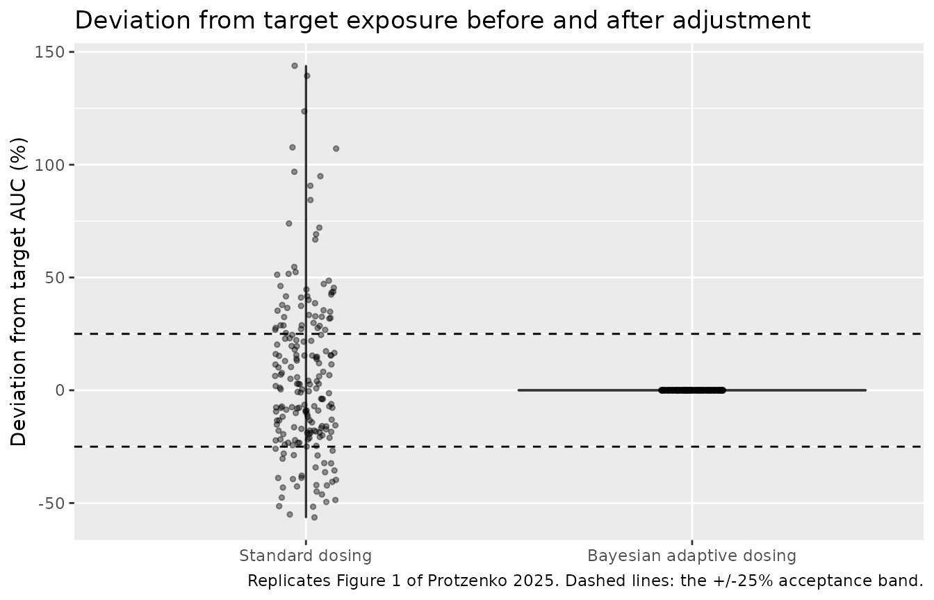
The standard-dose column is the out-of-sample part of this check: the deviation after a 3 mg/kg dose depends only on the prior’s distribution of clearance and on the cohort’s weight distribution. The simulated spread is wider than the published one (a mean absolute deviation of 27.4% against 19.5%, and a largest overshoot of 144% against 60.1%). That is expected from two things the simulation does not reproduce. The prior has no effect of body weight on clearance, so under a strict mg/kg dose the first-dose AUC is proportional to weight and the heaviest virtual patients overshoot most. And in the clinic the 3 mg/kg starting dose was modified for extreme weight, comorbidity, age or performance status: the starting doses ranged only from 126 to 294 mg (1.6-4.0 mg/kg), against 120-405 mg for a strict 3 mg/kg dose over the 40-135 kg weight range.
The adjusted column is not a reproduction of the paper’s 11.7%: the packaged model, like the paper’s prior, assumes that each patient’s clearance stays constant across the course, so an error-free adjustment lands on target exactly. The paper attributes its residual deviation to exactly the variability this model does not contain – a change of more than 20% in clearance between the first and last dose in a third of the patients (a mean decrease of 27% in 16 patients, a mean increase of 43% in 7) – together with the estimation error of a three-sample Bayesian fit.
Assumptions and deviations
-
Additive-normal random effects. The prior is
Gaussian on
1/Vandk, so the model addsetavcinvto1/Vandetakeltok. Normal random effects can in principle produce a non-positive value; here the means sit 5.1 and 10.6 standard deviations above zero, so this never occurs in practice. Because the eta onkis additive, the convention checker’s suggestion to rename itetalkelwould mislabel it as a log-scale effect, and the nameetakelis kept. -
Residual error held at zero. The first-stage fits
used a proportional error variance model, but the paper reports neither
its magnitude nor the error model of the Bayesian step.
propSdis held at 0, so simulated concentrations are individual predictions. The bioanalytical method has precision and accuracy within 15%. - Prior cohort demographics. The paper does not report the age, weight or dosing of the 16 patients behind the prior; the virtual cohort above follows the 71-patient application cohort (Table 1).
- Rich-sampling design. The Methods describe eight samples per patient from 2 to 12 h; the Discussion describes the same protocol as six samples.
- AUC unit conversion. The paper prints the targets as 66.0, 82.6 and 87.6 mg*h/L for 16 000, 20 000 and 21 200 uM*min. With a busulfan molar mass of 246.3 g/mol the conversions are 65.7, 82.1 and 87.0 mg*h/L; the printed values are used.
-
Cumulative AUC formula. The Methods print the
cumulative AUC as
AUC1 + (n - 2) * AUClast, which counts one administration fewer thann. The simulation sums the per-interval AUCs of all four doses directly. - Simulated regimen. Only the four-dose regimen (60 of 71 patients) is simulated; every simulated patient starts at exactly 3 mg/kg (the cohort’s actual starting doses averaged 2.9 mg/kg, range 1.6-4.0, at the clinician’s discretion). The single patient with an 18 000 uM*min target is folded into the 20 000 uM*min arm.
- Bayesian estimation. The first-dose NCA stands in for the Kinetic Pro Bayesian estimate, so the adjustment uses each simulated patient’s true clearance. The paper’s estimates had standard errors below 20%.