Daprodustat dose-hemoglobin response in anemia of CKD (Mahar 2025)
Source:vignettes/articles/Mahar_2025_daprodustat.Rmd
Mahar_2025_daprodustat.RmdModel and source
mod <- readModelDb("Mahar_2025_daprodustat")
ui <- rxode2::rxode(mod)
#> ℹ parameter labels from comments will be replaced by 'label()'
#> Warning: some etas defaulted to non-mu referenced, possible parsing error: etarbase, etarbase_true, etabvv_kprog_1, etabvv_kprog_2, etabvv_kprog_3
#> as a work-around try putting the mu-referenced expression on a simple line- Citation: Mahar KM, Yang S, Visser S, van Noort M, van den Berg P, Post TM. Integrated Longitudinal Population Dose-Hemoglobin Response of Daprodustat Following Dose Titration in Patients With Anemia in Chronic Kidney Disease. Clin Pharmacol Ther. 2025;117(3):846-855. doi:10.1002/cpt.3544
- Description: Longitudinal dose-hemoglobin model of daprodustat in adults with anemia of chronic kidney disease, fitted to five global phase III studies (Mahar 2025, Dose-Hgb Model 3). The current daprodustat dose level, allometrically scaled by baseline body weight, stimulates the production rate of a precursor-cell compartment through a power function (1 + SLOPE * dose^GAMMA, with GAMMA proportional to SLOPE). Precursors (mean transit t 3.19 days, fixed) mature into twelve red-cell age compartments whose transit times sum to the red-cell lifespan (82.8 days, fixed, with covariate effects), and total hemoglobin is the sum of the twelve age compartments. Hemoglobin production declines exponentially toward a (possibly negative) floor with a disease progression rate that depends on dialysis status and prior ESA use and has year-specific random effects for the first, second and later years. Prior ESA users start at an ESA-elevated apparent baseline and wash out to a separately estimated true baseline. Patient-group-specific baselines (non-dialysis, hemodialysis, peritoneal dialysis, starting dialysis) with CKD stage, body weight, baseline hepcidin, race, prior ESA dose and ESA hyporesponder effects; study-specific additive residual error on hemoglobin (g/L).
- Article: https://doi.org/10.1002/cpt.3544
- PubMed Central (with the supplementary NONMEM control stream): https://www.ncbi.nlm.nih.gov/pmc/articles/PMC11835430/
Daprodustat is an oral hypoxia-inducible factor prolyl hydroxylase
inhibitor. Mahar 2025 recalibrates GSK’s earlier dose-hemoglobin
(Dose-Hgb) models on the five global phase III studies (“Dose-Hgb Model
3”). The model is driven by the dose level, not by
concentrations: the paper notes that the red-cell lifespan (~82 days) is
far longer than the daprodustat half-life (1-4 h), and that oral
clearance was no better a predictor of response than dose. The current
dose level, divided by (WT / 73.3)^0.75, stimulates
precursor production through 1 + SLOPE * dose^GAMMA;
precursors mature through twelve red-cell age compartments, and
hemoglobin is their sum.
Because the dose enters as a time-varying covariate
(DOSE_DAPRODUSTAT_MG), a simulation needs no dosing events:
every row carries the dose level in force at that time.
Population
The analysis data set A contained 2,770 adults with anemia of chronic kidney disease (CKD) and 53,535 hemoglobin observations from five phase III studies (Mahar 2025 Table 1, Table S4, Table S7):
| Study | Population | Regimen | N (data set A) |
|---|---|---|---|
| 205270 | non-dialysis (ND), ESA non-users | QD, placebo-controlled | 205 |
| 204837 | hemodialysis (HD), ESA users | three times weekly (t.i.w.) | 180 |
| 201410 | starting HD (83) or PD (22), ESA non-users | QD | 105 |
| 200807 | HD (877) or PD (111), ESA users | QD | 988 |
| 200808 | ND, ESA non-users (683) and users (609) | QD | 1292 |
Median age was 63 years (range 17-96) and median body weight 73 kg (36-194); 54% were not on dialysis. Treatment lasted from 28 weeks to about 4 years, with the dose titrated to a hemoglobin target of 10-11 g/dL (11-12 g/dL in study 205270). Table S7 lists 1,484 males (50%) and 1,701 non-dialysis subjects (57%), neither of which matches its own per-study counts (1,396 males; 205 + 1,292 = 1,497 non-dialysis), so the per-study counts are used here.
str(mod()$population)
#> Warning: some etas defaulted to non-mu referenced, possible parsing error: etarbase, etarbase_true, etabvv_kprog_1, etabvv_kprog_2, etabvv_kprog_3
#> as a work-around try putting the mu-referenced expression on a simple line
#> List of 15
#>  $ species       : chr "human"
#>  $ n_subjects    : int 2770
#>  $ n_studies     : int 5
#>  $ n_observations: int 53535
#>  $ age_range     : chr "17-96 years"
#>  $ age_median    : chr "63 years"
#>  $ weight_range  : chr "36-194 kg"
#>  $ weight_median : chr "73 kg"
#>  $ sex_female_pct: num 50
#>  $ race_ethnicity: chr "White 62%, Asian 18%, Black 13%, American Indian / Alaska Native 4% (Table S7 percentages as printed)"
#>  $ disease_state : chr "Adults with anemia of chronic kidney disease: non-dialysis (ND) ESA non-users (studies 205270, 200808) and ESA "| __truncated__
#>  $ renal_function: chr "Non-dialysis 1497 (54%; CKD stages 2-5), hemodialysis 1140 (41%), peritoneal dialysis 133 (5%)"
#>  $ dose_range    : chr "Daprodustat titrated to a hemoglobin target (10-11 g/dL; 11-12 g/dL in study 205270): once daily 1-24 mg, or th"| __truncated__
#>  $ regions       : chr "Global (five pivotal phase III studies)"
#>  $ notes         : chr "Table S7 sex and race counts do not add up to N; the printed percentages are used. Analysis data set A: a rando"| __truncated__
Source trace
Every value comes from Mahar 2025 Table 2 (final model) and every equation from the NONMEM control stream printed in the Supplementary Methods (“NONMEM Code for Final Dose-Hgb Model”).
| Equation / parameter | Value | Source location |
|---|---|---|
rbase_nd_esanaive, rbase_nd_esa,
rbase_hd_esa, rbase_pd_esa
|
93.3, 103, 105, 103 g/L | Table 2; control stream THETA(1)-THETA(4) |
rbase_hd_start, rbase_pd_start
|
95.5, 101 g/L | Table 2; THETA(5)-THETA(6) |
rbase_true_nd_esa,
rbase_true_dial_esa
|
95.3, 94.9 g/L | Table 2; THETA(7)-THETA(8) |
e_esad_rbase_true |
-0.00797 | Table 2; PEPL = EXP((THETA(9)/1000) * PEPOD2)
|
e_esa_hyporesponder_rbase |
-0.0307 | Table 2; BLHYP = 1 + THETA(10)
|
e_chronic_kidney_disease_stage_rbase,
e_wt_rbase, e_hepcidin_bl_rbase
|
-0.107, 0.0520, -0.0170 | Table 2; BLSTAG, BLWT, BLHEP with medians 5, 73.3 kg, 121.356 ng/mL |
e_race_asian_rbase_true,
e_race_black_rbase
|
-0.0467, -0.0376 | Table 2; RACE_TBSL, RACE_BBSL |
lmtt, lmtt_rbc
|
log(3.19), log(82.819), both fixed | Table 2 (Fixed); THETA(16), THETA(17) |
e_esa_mtt_rbc, e_wt_mtt_rbc,
e_hd_mtt_rbc, e_study_201410_mtt_rbc
|
0.100, 0.271, 0.138, 0.309 | Table 2; EPO_TRBC, WTBL_TRBC, POP_TRBC |
lslope, gamma_slope_ratio,
e_race_black_slope
|
log(0.0580), 14.9, -0.128 | Table 2; SLOPE, GAMMA = corGAMMA * SLOPE,
RACE_SLP |
e_wt_dose |
0.75 (fixed) | Table 2; WTSL = (WTBL/medWtbl)**THETA(25)
|
e_study_204837_slope |
0.422 | Table 2; TIW = THETA(26) for study 204837 |
e_conmed_clopidogrel_dose |
-0.102 | Table 2; CLOP_DOSE
|
kprog, kin_min
|
-0.0851 per 1000 days, -0.678 g/L/day | Table 2; THETA(28), THETA(29) |
e_esa_kprog, e_dial_kprog,
e_study_201410_kprog
|
-0.318, -0.573, 0.968 | Table 2; EPO_DISPR, POP_DISPR |
e_study_205270_etarbase,
e_study_201410_etarbase
|
0.729, 1.13 | Table 2; OM1F |
etarbase + etarbase_true |
50.1, 40.3, 131 | Table 2 (variance, covariance, variance) |
etalslope, etalmtt_rbc
|
0.0280, 0.206 | Table 2 |
etabvv_kprog_1..3 block |
0.0504; 0.0212, 0.0178; 0.0121, 0.0108, 0.0104 | Table 2 |
addSd, addSd_205270,
addSd_204837, addSd_201410,
addSd_200808
|
7.27, 5.72, 6.28, 7.24, 6.39 g/L | Table 2 (study 200807 is the reference) |
| Precursor and 12 red-cell age compartments | n/a | Supplementary Methods Equations 1, 4-7; control stream $DES |
| Production with disease progression | n/a | Main text Equation 1; Supplementary Equation 2;
PROD = (KIN-MINKIN)*EXP(DISPR*T) + MINKIN, floored at
0 |
| Drug effect | n/a | Supplementary Equation 3;
EFF = 1 + SLOPE * (DDR**GAMMA) * TIW
|
| Initial conditions | n/a | Supplementary Methods (“Steady state without drug”); control stream A_0 |
Typical subjects
The helper below builds one row per observation time for a typical subject of each patient group. Unless stated otherwise, covariates sit at the model’s reference values (weight 73.3 kg, hepcidin 121.356 ng/mL), non-dialysis subjects are CKD stage 4 and dialysis subjects stage 6 (the paper’s dialysis stage), and ESA users carry the Table S8 reference prior ESA dose of 5,275 IU/week.
mod_typ <- rxode2::zeroRe(mod)
#> ℹ parameter labels from comments will be replaced by 'label()'
#> Warning: some etas defaulted to non-mu referenced, possible parsing error: etarbase, etarbase_true, etabvv_kprog_1, etabvv_kprog_2, etabvv_kprog_3
#> as a work-around try putting the mu-referenced expression on a simple line
#> Warning: No sigma parameters in the model
#> Warning: some etas defaulted to non-mu referenced, possible parsing error: etarbase, etarbase_true, etabvv_kprog_1, etabvv_kprog_2, etabvv_kprog_3
#> as a work-around try putting the mu-referenced expression on a simple line

groups <- tibble::tribble(
  ~group,                                 ~RRT_HEMODIAL_STATUS, ~PERIT_DIAL, ~ESAD, ~CHRONIC_KIDNEY_DISEASE_STAGE, ~STUDY_201410, ~STUDY_200808,
  "No dialysis, ESA non-user",            0,                    0,           0,     4,          0,             1,
  "No dialysis, ESA user",                0,                    0,           5275,  4,          0,             1,
  "HD, ESA user",                         1,                    0,           5275,  6,          0,             0,
  "PD, ESA user",                         0,                    1,           5275,  6,          0,             0,
  "Just started HD, ESA non-user",        1,                    0,           0,     6,          1,             0
) |>
  mutate(
    id = row_number(), WT = 73.3, HEPCIDIN_BL = 121.356, ESA_HYPORESPONDER = 0,
    RACE_BLACK = 0, RACE_ASIAN = 0, CONMED_CLOPIDOGREL = 0,
    STUDY_205270 = 0, STUDY_204837 = 0
  )

make_events <- function(subjects, times, dose = 0) {
  tidyr::expand_grid(id = subjects$id, time = times) |>
    left_join(subjects, by = "id") |>
    mutate(evid = 0, cmt = "hb1", DOSE_DAPRODUSTAT_MG = dose)
}
Disease progression (Figure 4)
Without treatment, precursor production declines as
(kin - kin_min) * exp(dispr * t) + kin_min. Figure 4 of
Mahar 2025 plots the factor exp(dispr * t) for the typical
subject of each group. The model returns dispr (per day)
for every subject, so the figure follows directly from the
simulation.
sim_dp <- rxode2::rxSolve(mod_typ, make_events(groups, seq(0, 4 * 365.25, by = 7)),
  returnType = "data.frame", keep = "group"
) |>
  mutate(dp_factor = exp(dispr * time), year = time / 365.25) |>
  filter(group != "PD, ESA user", !(group == "Just started HD, ESA non-user" & year > 1))
#> ℹ omega/sigma items treated as zero: 'etarbase', 'etarbase_true', 'etalslope', 'etalmtt_rbc', 'etabvv_kprog_1', 'etabvv_kprog_2', 'etabvv_kprog_3'
#> Warning: multi-subject simulation without without 'omega'

ggplot(sim_dp, aes(year, dp_factor, colour = group)) +
  geom_line(linewidth = 1) +
  labs(x = "Time (year)", y = "Disease progression factor (-)", colour = NULL) +
  theme_bw()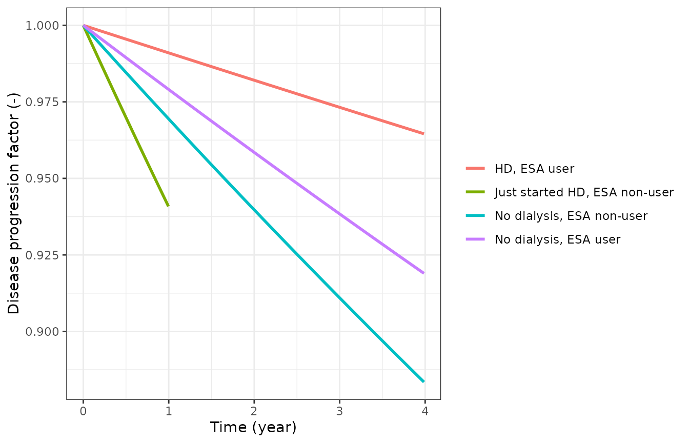
Replicates Figure 4 of Mahar 2025. The values at the end of each curve, read from the published figure, agree with the model:
fig4 <- tibble::tribble(
  ~group,                          ~year, ~published,
  "No dialysis, ESA non-user",     4,     0.883,
  "No dialysis, ESA user",         4,     0.919,
  "HD, ESA user",                  4,     0.964,
  "Just started HD, ESA non-user", 1,     0.941
)
fig4_check <- fig4 |>
  rowwise() |>
  mutate(model = exp(sim_dp$dispr[sim_dp$group == group][1] * year * 365.25)) |>
  ungroup()
fig4_check |>
  dplyr::rename("Group" = group, "Year" = year, "Figure 4 (read)" = published, "Model" = model) |>
knitr::kable(digits = 3)| Group | Year | Figure 4 (read) | Model |
|---|---|---|---|
| No dialysis, ESA non-user | 4 | 0.883 | 0.883 |
| No dialysis, ESA user | 4 | 0.919 | 0.919 |
| HD, ESA user | 4 | 0.964 | 0.964 |
| Just started HD, ESA non-user | 1 | 0.941 | 0.941 |
Effect of disease progression on hemoglobin (Table S9)
Table S9 reports the reduction in steady-state hemoglobin after one
year without daprodustat, for a typical subject starting at 10 g/dL (100
g/L). At steady state hemoglobin equals production times lifespan, so
the reduction is 100 * (prod(365) / kin - 1) with
kin = 100 / lifespan.
theta <- ui$theta
s9 <- sim_dp |>
  filter(time == 0, group != "PD, ESA user") |>
  select(group, dispr, mtt_rbc)
s9 <- s9 |>
  mutate(
    kin_ref = 100 / exp(theta[["lmtt_rbc"]]),
    delta_ref = 100 * (((kin_ref - theta[["kin_min"]]) * exp(dispr * 365) + theta[["kin_min"]]) / kin_ref - 1),
    kin_cov = 100 / mtt_rbc,
    delta_cov = 100 * (((kin_cov - theta[["kin_min"]]) * exp(dispr * 365) + theta[["kin_min"]]) / kin_cov - 1),
    published = c(-4.8, -3.3, -1.4, -9.3)
  )
s9 |>
  select(group, published, delta_ref, delta_cov) |>
  dplyr::rename(
    "Group" = group, "Table S9 (g/L/year)" = published,
    "Model, lifespan 82.8 days" = delta_ref,
    "Model, covariate-adjusted lifespan" = delta_cov
  ) |>
knitr::kable(digits = 2)| Group | Table S9 (g/L/year) | Model, lifespan 82.8 days | Model, covariate-adjusted lifespan |
|---|---|---|---|
| No dialysis, ESA non-user | -4.8 | -4.78 | -4.78 |
| No dialysis, ESA user | -3.3 | -3.27 | -3.39 |
| HD, ESA user | -1.4 | -1.41 | -1.53 |
| Just started HD, ESA non-user | -9.3 | -9.26 | -10.29 |
# Same closed form on both sides; the tolerance covers Table S9's rounding
# to 0.1 g/L.
stopifnot(all(abs(s9$delta_ref - s9$published) < 0.06))
The table is reproduced exactly when every group uses the reference red-cell lifespan of 82.8 days. With the covariate-adjusted lifespan (+13.8% for HD, +30.9% for subjects starting dialysis, +10% for ESA users) the HD and starting-dialysis rows become -1.5 and -10.3 g/L. Table S9 was therefore computed with the reference lifespan, which the paper does not state.
ESA washout
ESA users enter at an apparent, ESA-elevated baseline (105 g/L for a typical HD ESA user) and, once the ESA is replaced by daprodustat at the first dose, drift to their true baseline over roughly one red-cell lifespan. Without daprodustat the typical HD ESA user settles near the true baseline:
sim_wash <- rxode2::rxSolve(mod_typ, make_events(groups, seq(0, 365, by = 3)),
  returnType = "data.frame", keep = "group"
)
#> ℹ omega/sigma items treated as zero: 'etarbase', 'etarbase_true', 'etalslope', 'etalmtt_rbc', 'etabvv_kprog_1', 'etabvv_kprog_2', 'etabvv_kprog_3'
#> Warning: multi-subject simulation without without 'omega'

ggplot(sim_wash, aes(time, hb, colour = group)) +
  geom_line(linewidth = 1) +
  labs(x = "Time since first dose (day)", y = "Hemoglobin (g/L)", colour = NULL,
       caption = "No daprodustat (dose level 0)") +
  theme_bw()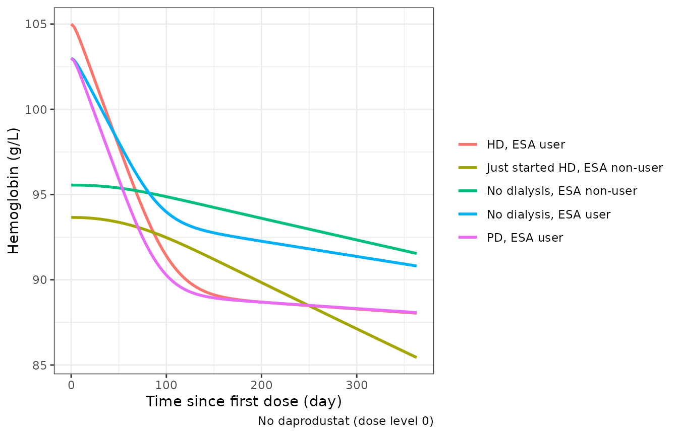
hd <- sim_wash[sim_wash$group == "HD, ESA user", ]
stopifnot(
  abs(hd$hb[hd$time == 0] - theta[["rbase_hd_esa"]]) < 1e-6,
  # After ~2 lifespans the chain has turned over; only the slow disease
  # progression (about 1.4 g/L per year) separates hb from the true baseline.
  abs(hd$hb[hd$time == 183] - hd$rbase_true[1]) < 2
)
Dose response and the t.i.w. factor
Typical non-dialysis ESA non-users held at a fixed daprodustat dose for one year (the studies titrated the dose; this only shows the shape of the dose response):
nd <- groups[groups$group == "No dialysis, ESA non-user", ]
doses <- c(0, 1, 2, 4, 8)
sim_dr <- bind_rows(lapply(seq_along(doses), function(i) {
  ev <- make_events(mutate(nd, id = i), seq(0, 364, by = 7), dose = doses[i])
  rxode2::rxSolve(mod_typ, ev, returnType = "data.frame") |>
    mutate(dose = factor(paste(doses[i], "mg QD"), levels = paste(doses, "mg QD")))
}))
#> ℹ omega/sigma items treated as zero: 'etarbase', 'etarbase_true', 'etalslope', 'etalmtt_rbc', 'etabvv_kprog_1', 'etabvv_kprog_2', 'etabvv_kprog_3'
#> ℹ omega/sigma items treated as zero: 'etarbase', 'etarbase_true', 'etalslope', 'etalmtt_rbc', 'etabvv_kprog_1', 'etabvv_kprog_2', 'etabvv_kprog_3'
#> ℹ omega/sigma items treated as zero: 'etarbase', 'etarbase_true', 'etalslope', 'etalmtt_rbc', 'etabvv_kprog_1', 'etabvv_kprog_2', 'etabvv_kprog_3'
#> ℹ omega/sigma items treated as zero: 'etarbase', 'etarbase_true', 'etalslope', 'etalmtt_rbc', 'etabvv_kprog_1', 'etabvv_kprog_2', 'etabvv_kprog_3'
#> ℹ omega/sigma items treated as zero: 'etarbase', 'etarbase_true', 'etalslope', 'etalmtt_rbc', 'etabvv_kprog_1', 'etabvv_kprog_2', 'etabvv_kprog_3'

ggplot(sim_dr, aes(time / 7, hb, colour = dose)) +
  geom_line(linewidth = 1) +
  labs(x = "Week", y = "Hemoglobin (g/L)", colour = NULL) +
  theme_bw()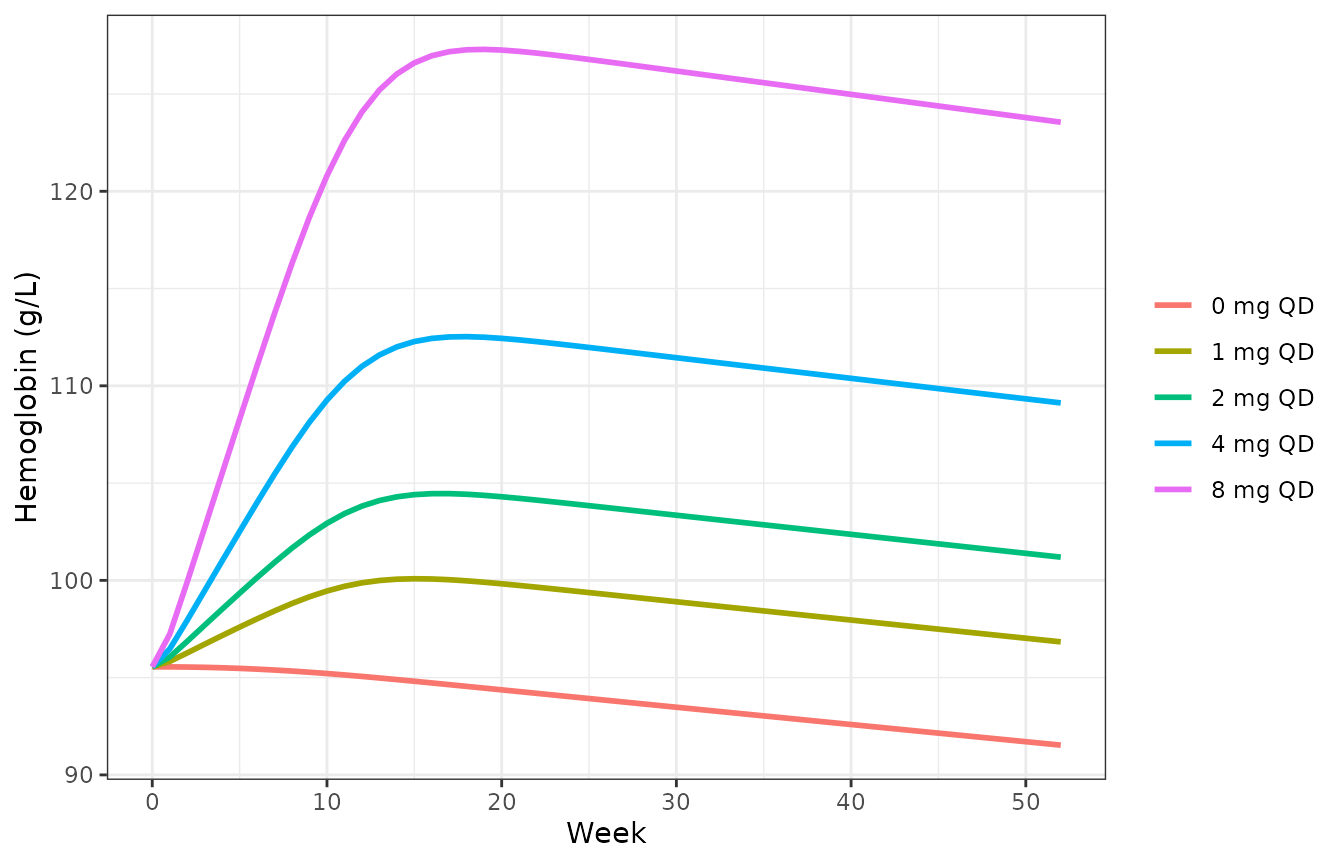
In study 204837 daprodustat was given three times weekly and the dose level is the per-administration dose. The estimated factor on the effect, 0.422, is close to 3/7 = 0.429, the value expected if the response follows the average daily dose with a linear dose term. Because GAMMA is below 1 (0.864 for a typical subject), a weekly-dose-matched t.i.w. regimen (7/3 times the QD dose) gives a slightly smaller effect than QD:
hd_esa <- groups[groups$group == "HD, ESA user", ]
ev_tiw <- bind_rows(
  make_events(mutate(hd_esa, id = 1), c(1, 182), dose = 4),
  make_events(mutate(hd_esa, id = 2, STUDY_204837 = 1), c(1, 182), dose = 4 * 7 / 3)
)
sim_tiw <- rxode2::rxSolve(mod_typ, ev_tiw, returnType = "data.frame")
#> ℹ omega/sigma items treated as zero: 'etarbase', 'etarbase_true', 'etalslope', 'etalmtt_rbc', 'etabvv_kprog_1', 'etabvv_kprog_2', 'etabvv_kprog_3'
#> Warning: multi-subject simulation without without 'omega'
eff_ratio <- (sim_tiw$eff[sim_tiw$id == 2][1] - 1) / (sim_tiw$eff[sim_tiw$id == 1][1] - 1)
gamma_typ <- theta[["gamma_slope_ratio"]] * exp(theta[["lslope"]])
eff_ratio
#> [1] 0.8776432
stopifnot(abs(eff_ratio - theta[["e_study_204837_slope"]] * (7 / 3)^gamma_typ) < 1e-6)
sim_tiw |> filter(time == 182) |> select(id, hb)
#>   id       hb
#> 1  1 105.8044
#> 2  2 103.7224
Stochastic simulation
A virtual cohort of 100 non-dialysis ESA non-users per arm (study 200808 residual error, CKD stage 3-5, body weight log-normal around 73 kg), treated with a fixed 0, 2 or 4 mg QD for one year:
set.seed(2025)
n_per_arm <- 100
arms <- c(0, 2, 4)
cohort <- bind_rows(lapply(seq_along(arms), function(i) {
  tibble(
    id = (i - 1) * n_per_arm + seq_len(n_per_arm),
    arm = paste(arms[i], "mg QD"),
    DOSE_DAPRODUSTAT_MG = arms[i],
    WT = pmin(pmax(exp(rnorm(n_per_arm, log(73), 0.22)), 40), 160),
    CHRONIC_KIDNEY_DISEASE_STAGE = sample(3:5, n_per_arm, replace = TRUE, prob = c(0.2, 0.5, 0.3)),
    HEPCIDIN_BL = exp(rnorm(n_per_arm, log(121), 0.6)),
    RACE_BLACK = rbinom(n_per_arm, 1, 0.13),
    RACE_ASIAN = 0
  )
})) |>
  mutate(
    RACE_ASIAN = ifelse(RACE_BLACK == 0, rbinom(n(), 1, 0.2), 0),
    ESAD = 0, ESA_HYPORESPONDER = 0, RRT_HEMODIAL_STATUS = 0, PERIT_DIAL = 0,
    CONMED_CLOPIDOGREL = 0, STUDY_205270 = 0, STUDY_204837 = 0,
    STUDY_201410 = 0, STUDY_200808 = 1
  )
events <- tidyr::expand_grid(id = cohort$id, time = seq(0, 364, by = 14)) |>
  left_join(cohort, by = "id") |>
  mutate(evid = 0, cmt = "hb1")

rxode2::rxSetSeed(2025)
sim <- rxode2::rxSolve(mod, events, returnType = "data.frame", keep = "arm")
#> ℹ parameter labels from comments will be replaced by 'label()'
#> Warning: some etas defaulted to non-mu referenced, possible parsing error: etarbase, etarbase_true, etabvv_kprog_1, etabvv_kprog_2, etabvv_kprog_3
#> as a work-around try putting the mu-referenced expression on a simple line

sim_sum <- sim |>
  group_by(arm, time) |>
  summarise(
    q05 = quantile(sim, 0.05), q50 = median(sim), q95 = quantile(sim, 0.95),
    .groups = "drop"
  )
ggplot(sim_sum, aes(time / 7, q50, colour = arm, fill = arm)) +
  geom_ribbon(aes(ymin = q05, ymax = q95), alpha = 0.15, colour = NA) +
  geom_line(linewidth = 1) +
  geom_hline(yintercept = c(100, 110), linetype = 2) +
  labs(x = "Week", y = "Hemoglobin (g/L)", colour = NULL, fill = NULL,
       caption = "Median and 90% prediction interval; dashed lines: 10-11 g/dL target") +
  theme_bw()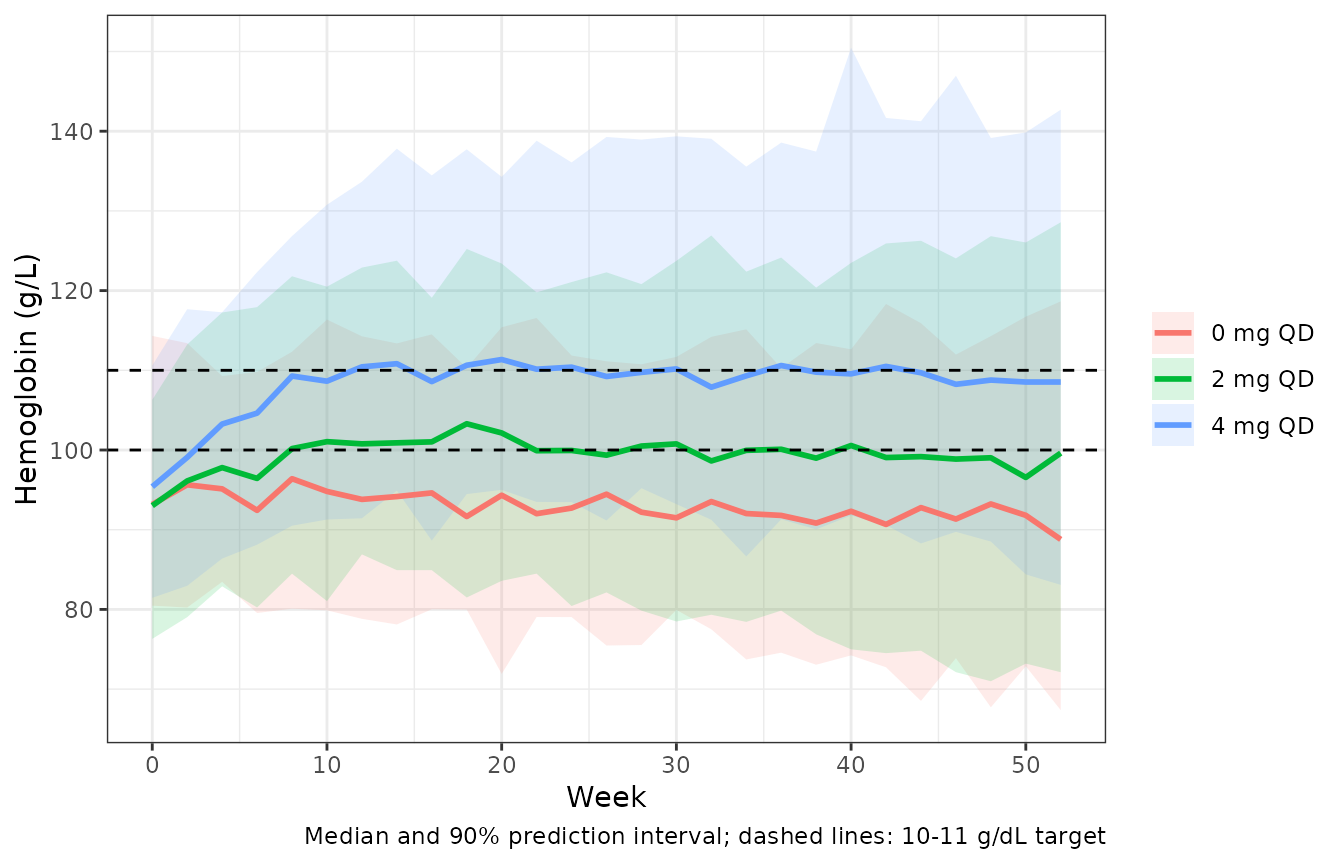
base_med <- median(sim$sim[sim$time == 0])
wk52 <- sim |>
  filter(time == max(time)) |>
  group_by(arm) |>
  summarise(median_hb = median(sim))
wk52
#> # A tibble: 3 × 2
#>   arm     median_hb
#>   <chr>       <dbl>
#> 1 0 mg QD      88.8
#> 2 2 mg QD      99.6
#> 3 4 mg QD     109.
stopifnot(
  # Centre of the cohort baseline near the typical ND ESA non-user value
  # (93.3 g/L, modulated by CKD stage and hepcidin).
  abs(base_med - 95) < 4,
  # A 4 mg QD dose raises the cohort median by well over the residual SD.
  wk52$median_hb[wk52$arm == "4 mg QD"] - wk52$median_hb[wk52$arm == "0 mg QD"] > 8
)
PKNCA
The model has no drug concentrations: it is driven directly by the dose level, so there is no exposure to summarise by non-compartmental analysis and no published NCA to compare with. PKNCA is therefore not used.
Assumptions and deviations
-
Time origin. Time is days since the first
daprodustat dose. The control stream used the study day (day 1 = first
dose) for the switch from the apparent to the true baseline and for the
disease-progression exponent; the one-day shift is negligible against a
red-cell lifespan of 83 days and a progression rate of 0.0000851 per
day. The year-specific random effects switch at 367 and 732 days after
the first dose, as coded (
RTFD8808 h and 17568 h). -
ESA-user flag. The control stream carries a
separate prior-ESA category (EPO: none, historic, recent); historic and
recent users were modelled identically. Here
ESAD > 0marks an ESA user, and the flag is forced to 0 in studies 205270 and 201410 as in the control stream. ESA users with an unrecorded prior dose should carry the control stream’s imputed value, 71.299 IU/kg/week times body weight. -
Starting dialysis and t.i.w. dosing are study
indicators. The control stream assigns the “just started /
starting dialysis” population by study
(
IF(STUDYID.EQ.201410) POP = 4) and the t.i.w. factor by study (IF(STUDYID.EQ.204837) TIW = THETA(26)); the model keeps those study indicators, which also select the study-specific residual SD and apparent-baseline variability. -
The t.i.w. factor multiplies the effect. Table 2
calls it a “factor on CDOSE”, but the control stream applies it to the
effect term (
EFF = 1 + SLOPE * (DDR**GAMMA) * TIW); the control stream is followed. - Undefined patient groups. No baseline was estimated for chronic dialysis ESA non-users or for ESA users starting dialysis, because no such subjects were studied; the model gives a typical apparent baseline of 0 for them and should not be used there.
- Black race on the apparent baseline. Table 2 lists the Black-race effect on the “true and apparent baseline”; in the control stream it reaches the apparent baseline only for ESA non-users (whose apparent and true baselines coincide) and the true baseline of ESA users. The control stream is followed.
- Lifespans. The red-cell lifespan is fixed at 82.819 days, the control stream value that Table 2 rounds to 82.8.
- Titration not reproduced. The paper’s visual predictive checks (Figures 2 and 3, Table 3) titrate each simulated subject’s dose by the study algorithms of Table S3. The available dose steps are not listed in the paper, so the titration VPCs are not reproduced; the simulations above use fixed doses.
- Table S9 reproduces only with the reference red-cell lifespan for every group, as shown above.
- Virtual-cohort covariates. The hepcidin, CKD-stage and race distributions of the stochastic cohort are approximations; Table S7 gives only means and percentages, and some of its counts do not add up.