Milrinone (O'Hanlon 2024)
Source:vignettes/articles/OHanlon_2024_milrinone.Rmd
OHanlon_2024_milrinone.RmdModel and source
- Citation: O’Hanlon CJ, Sumpter A, Anderson BJ, Hannam JA. Time-Varying Clearance in Milrinone Pharmacokinetics from Premature Neonates to Adolescents. Clin Pharmacokinet. 2024;63(5):695-706. doi:10.1007/s40262-024-01372-5
- Description: One-compartment population PK model of intravenous milrinone from premature neonates to adolescents (O’Hanlon 2024), pooling 50 children after cardiac surgery with cardiopulmonary bypass and 29 very premature neonates (Paradisis 2007). Clearance scales with fat-free mass (exponent 3/4), a sigmoid postmenstrual-age maturation function and relative renal function (eGFR / normal GFR), and rises over time on milrinone from 63.7% of its asymptote at infusion start (fractional deficit 0.363, half-time 11.9 h). Volume scales linearly with fat-free mass and is 2.06 times its mature value at birth, decaying toward it with a postnatal-age half-time of 0.969 days. Correlated log-normal IIV on CL and V; combined residual error estimated separately for two LC-MS bioanalytical batches and the HPLC-UV neonatal study, with a log-normal random effect on the residual SD.
- Article: https://doi.org/10.1007/s40262-024-01372-5 (open access; PMC11106138)
- Supplement: electronic supplementary material 1 (Tables S1-S2, VPC and simulation figures) and 2 (the final-model NONMEM control stream), both linked from the article page.
No erratum or correction notice for this article was found on the publisher page or in PubMed as of 2026-11-08.
Population
O’Hanlon 2024 pooled two studies (Table 1). The Starship Children’s Hospital study (Auckland, New Zealand, 2011-2012) enrolled 50 children aged 4 days to 16 years (median postnatal age 0.656 years, median weight 8.05 kg, 3.44-80.9 kg; 60% male) who received a milrinone infusion of 0.25-1.25 ug/kg/min after cardiac surgery with cardiopulmonary bypass, titrated to response. Plasma milrinone was measured by LC-MS (LLOQ 5 ug/L) in two analytical batches; 37 of 245 samples were below the LLOQ and were handled with the M3 method. Paradisis et al. 2007 contributed 29 very premature neonates (postmenstrual age 23.7-27.3 weeks, postnatal age 0.125-1.25 days, median weight 0.85 kg) given 0.25, 0.5 or 0.75 ug/kg/min for 3 h followed by 0.2 ug/kg/min to prevent low systemic blood flow, with 124 serum samples measured by HPLC-UV (LLOQ 20 ug/L). Altogether 369 concentrations from 79 patients were analysed in NONMEM 7.5.1.
The same information is available programmatically:
str(rxode2::rxode(readModelDb("OHanlon_2024_milrinone"))$population)
#> ℹ parameter labels from comments will be replaced by 'label()'
#> List of 15
#>  $ species       : chr "human"
#>  $ n_subjects    : int 79
#>  $ n_studies     : int 2
#>  $ n_observations: int 369
#>  $ age_range     : chr "Starship study: PNA 4 days to 16 years (PMA 39.1-769 weeks, 2.5th-97.5th percentile); Paradisis 2007: PNA 0.125"| __truncated__
#>  $ age_median    : chr "Starship study: PNA 0.656 years, PMA 73.8 weeks; Paradisis 2007: PNA 0.75 days, PMA 26.0 weeks"
#>  $ weight_range  : chr "Starship study: 3.44-80.9 kg; Paradisis 2007: 0.549-1.17 kg (2.5th-97.5th percentile)"
#>  $ weight_median : chr "Starship study: 8.05 kg; Paradisis 2007: 0.85 kg"
#>  $ ffm_median    : chr "Starship study: 5.80 kg (3.02-54.6); Paradisis 2007: 0.808 kg (0.522-1.11)"
#>  $ sex_female_pct: num 40.5
#>  $ disease_state : chr "Starship study: children after cardiac surgery supported by cardiopulmonary bypass, milrinone for prophylaxis o"| __truncated__
#>  $ dose_range    : chr "Starship study: IV infusion 0.25-1.25 ug/kg/min started after the end of bypass, titrated to response; Paradisi"| __truncated__
#>  $ renal_function: chr "Day-1 eGFR median 54.1 mL/min/1.73 m^2 (18.1-93.3) in the Starship study; RF assumed 1 in Paradisis 2007 neonates."
#>  $ regions       : chr "New Zealand (Starship Children's Hospital, Auckland) and Australia (Paradisis 2007)."
#>  $ notes         : chr "O'Hanlon 2024 Table 1 and Results. 245 Starship samples (LC-MS, LLOQ 5 ug/L, two analytical batches; 37 BLQ han"| __truncated__
Source trace
Every ini() value carries an in-file comment pointing at
its source. All structural values appear in Table 2 and, identically, as
the $THETA of the published control stream (ESM 2), with
the one exception noted below.
| Equation / parameter | Value | Source location |
|---|---|---|
lcl (asymptotic CL, 70 kg / 56.1 kg FFM) |
log(17.6) L/h |
Table 2 ‘CL’; ctl POP_CL
|
lvc (mature V, 70 kg / 56.1 kg FFM) |
log(20.8) L |
Table 2 ‘V’; ctl POP_V
|
e_ffm_cl, e_ffm_vc
|
0.75, 1 (fixed) | Eq. 13-14; ctl FSZ_CL_RF, FSZ_V
|
| NFM = FFM, NFMstd = 56.1 kg | Ffat = 0 (fixed) | Eq. 1-3; Table 2 ‘Ffat CL’, ‘Ffat V’ = 0 FIX |
ltmat50 |
log(49.8) weeks PMA |
Table 2 ‘TM50’; ctl TM50_RF
|
lhill_mat |
log(4.04) |
Table 2 ‘HILL’; ctl HILL_RF
|
Maturation 1 / (1 + (PMA / TM50)^-HILL)
|
n/a | Eq. 4 |
RENALFUNC_REL multiplies CL |
n/a | Eq. 6, 13; ctl FRF (FCLR = 1 FIX) |
cl_exp_fdef |
0.363 | Table 2 ‘FCL’; ctl POP_CONCL
|
lcl_exp_kdes |
log(log(2) / 11.9) 1/h |
Table 2 ‘TCL’ = 11.9 h; ctl POP_TCL
|
cl(t) = cl * (1 - FCL * exp(-ln2 * t / TCL)), inside
the ODE |
n/a | Eq. 9, 13; ctl $DES
|
vc_pna_famp |
1.06 | Table 2 ‘FV’; ctl POP_CONV_PNA
|
lvc_pna_kdes |
log(log(2) / 0.969) 1/day |
Table 2 ‘TVOL’ = 0.969 days; ctl POP_TVOL_PNA
|
V = vc * (1 + FV * exp(-ln2 * PNA_days / TVOL)) |
n/a | Eq. 5, 14; ctl VAGE_PNA
|
etalcl + etalvc |
0.129, 0.114, 0.115 | ctl $OMEGA BLOCK(2); Table 2 PPV 0.359 / 0.339, r
0.936 |
etaRUV |
0.0669 | ctl PPV_RUVCP; Table 2 ‘PPV RUV’ 0.259 |
propSd, addSd (batch 1) |
0.382, 34.8 ug/L | Table 2 ‘CV / SD batch 1’; ctl RUV_CVCP1,
RUV_SDCP1
|
propSd_batch2, addSd_batch2
|
0.332, 7.86 ug/L | Table 2 ‘CV / SD batch 2’ (ctl RUV_CVCP2 = 0.322) |
propSd_paradisis, addSd_paradisis
|
0 (fixed), 31.4 ug/L | Table 2 ‘CV / SD Paradisis’; ctl RUV_CVCP3,
RUV_SDCP3
|
Combined error
sqrt((CP*CV)^2 + SD^2) * exp(etaRUV)
|
n/a | Eq. 12; ctl $ERROR
|
The PPVs reproduce from the OMEGA block:
sqrt(0.129) = 0.359, sqrt(0.115) = 0.339, and
0.114 / sqrt(0.129 * 0.115) = 0.936.
Time-varying clearance and the birth effect on volume (Figure 1)
Figure 1 of the paper shows the two empirical functions of the final
model. The chunk below evaluates them through the packaged model itself
(the model’s cl_time and vc outputs from a
typical-value solve) rather than from hand-written formulas.
mod <- readModelDb("OHanlon_2024_milrinone")
mod_typical <- rxode2::zeroRe(mod)
#> ℹ parameter labels from comments will be replaced by 'label()'
#> Warning: No sigma parameters in the model

# A 70 kg adult (FFM 56.1 kg, fully mature, normal renal function) per value
# of postnatal age in days; observation grid over 0-50 h.
pna_days <- seq(0, 8, by = 0.25)
fig1_ev <- tidyr::expand_grid(id = seq_along(pna_days), time = seq(0, 50, by = 0.5)) |>
  mutate(
    evid = 0, amt = 0, cmt = "central",
    PNA = pna_days[id] / 30.4375,
    FFM = 56.1, PAGE = 2000, RENALFUNC_REL = 1,
    ASSAY_BATCH2 = 0, STUDY_PARADISIS2007 = 0
  )
fig1 <- rxode2::rxSolve(mod_typical, events = fig1_ev) |>
  as.data.frame()
#> ℹ omega/sigma items treated as zero: 'etalcl', 'etalvc', 'etaRUV'
#> Warning: multi-subject simulation without without 'omega'

fcl <- fig1 |> filter(id == max(id))
fv <- fig1 |> filter(time == 0) |> mutate(pna_d = pna_days[id], fv = vc / 20.8)

stopifnot(
  # CL starts at 1 - 0.363 = 0.637 of its asymptote and has risen to 0.95
  # by 2.4 half-times (~29 h).
  abs(fcl$cl_time[fcl$time == 0] - 0.637) < 1e-9,
  abs(fcl$cl_time[fcl$time == 50] - (1 - 0.363 * 2^(-50 / 11.9))) < 1e-9,
  # V at birth is 1 + 1.06 = 2.06 times the mature value: 42.8 L / 70 kg.
  abs(fv$vc[fv$pna_d == 0] - 20.8 * 2.06) < 1e-9
)

p1 <- ggplot(fcl, aes(time, cl_time)) +
  geom_line() +
  labs(x = "Time after dose initiation (h)", y = "Fractional change in CL",
       title = "Time-varying CL")
p2 <- ggplot(fv, aes(pna_d, fv)) +
  geom_line() +
  labs(x = "PNA (days)", y = "Fractional change in V",
       title = "Birth effect on V")
print(p1)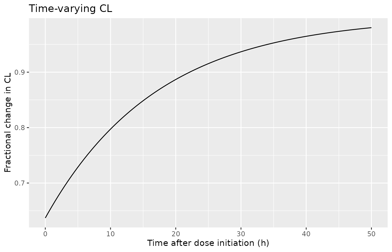
print(p2)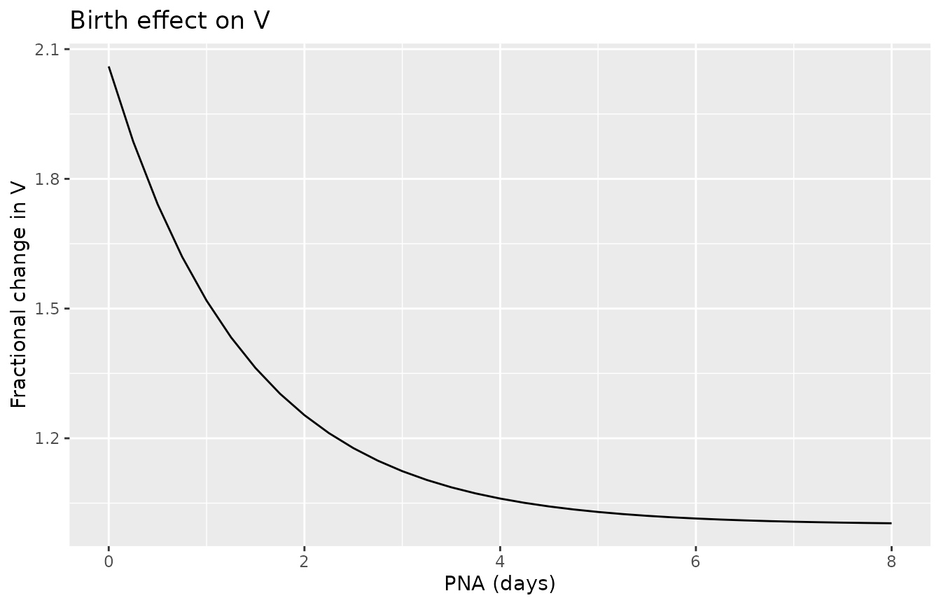
Replicates Figure 1 of O’Hanlon 2024: the left panel starts at 0.637 and approaches 1 by 50 h; the right panel starts at 2.06 and approaches 1 by PNA 6-8 days.
The Discussion quotes the volume at birth as 42.6 L/70 kg and at 1 day PNA as 31.2 L/70 kg. Those numbers use the bootstrap means (V 20.4 L, FV 1.07, TVOL 0.977 days); the final estimates packaged here give the values below.
v_check <- tibble(
  `PNA (days)` = c(0, 1),
  `Packaged model (final estimates), L/70 kg` = signif(
    approx(fv$pna_d, fv$vc, xout = c(0, 1))$y, 3
  ),
  `Bootstrap means, L/70 kg` = signif(20.4 * (1 + 1.07 * 2^(-c(0, 1) / 0.977)), 3),
  `Paper text, L/70 kg` = c(42.6, 31.2)
)
knitr::kable(v_check)| PNA (days) | Packaged model (final estimates), L/70 kg | Bootstrap means, L/70 kg | Paper text, L/70 kg |
|---|---|---|---|
| 0 | 42.8 | 42.2 | 42.6 |
| 1 | 31.6 | 31.1 | 31.2 |
Steady-state check and PKNCA
With CL fully recovered (t much greater than TCL), the
concentration during a constant-rate infusion approaches
rate / CL. A typical 70 kg adult at 0.5 ug/kg/min (2100
ug/h) with CL = 17.6 L/h should therefore average 119.3 ug/L over a late
dosing interval. PKNCA computes the average concentration over 168-192 h
of a continuous infusion.
rate_adult <- 0.5 * 70 * 60 # ug/h
ss_ev <- bind_rows(
  tibble(id = 1L, time = 0, evid = 1, amt = rate_adult * 200, rate = rate_adult, cmt = "central"),
  tibble(id = 1L, time = c(0, seq(0.5, 200, by = 0.5)), evid = 0, amt = 0, rate = 0, cmt = "central")
) |>
  mutate(
    FFM = 56.1, PAGE = 2000, PNA = 360, RENALFUNC_REL = 1,
    ASSAY_BATCH2 = 0, STUDY_PARADISIS2007 = 0, treatment = "0.5 ug/kg/min, 70 kg"
  ) |>
  arrange(id, time, desc(evid))
ss_sim <- rxode2::rxSolve(mod_typical, events = ss_ev, keep = "treatment",
                          rtol = 1e-10, atol = 1e-12) |>
  as.data.frame()
#> ℹ omega/sigma items treated as zero: 'etalcl', 'etalvc', 'etaRUV'
if (is.null(ss_sim$id)) ss_sim$id <- 1L

conc_df <- ss_sim |>
  filter(!is.na(Cc)) |>
  select(id, time, Cc, treatment)
dose_df <- ss_ev |>
  filter(evid == 1) |>
  mutate(duration = amt / rate) |>
  select(id, time, amt, duration, treatment)

conc_obj <- PKNCA::PKNCAconc(conc_df, Cc ~ time | treatment + id)
dose_obj <- PKNCA::PKNCAdose(dose_df, amt ~ time | treatment + id,
                             route = "intravascular", duration = "duration")
intervals <- data.frame(start = 168, end = 192, cav = TRUE, cmax = TRUE, cmin = TRUE)
nca_res <- PKNCA::pk.nca(PKNCA::PKNCAdata(conc_obj, dose_obj, intervals = intervals))

nca_tab <- as.data.frame(nca_res$result) |>
  select(treatment, PPTESTCD, PPORRES) |>
  tidyr::pivot_wider(names_from = PPTESTCD, values_from = PPORRES) |>
  mutate(closed_form = rate_adult / 17.6)
knitr::kable(
  nca_tab |>
    rename(
      Regimen = treatment, `Cav 168-192 h (ug/L)` = cav,
      `Cmax (ug/L)` = cmax, `Cmin (ug/L)` = cmin,
      `AUClast 168-192 h (ug*h/L)` = auclast,
      `rate / CL (ug/L)` = closed_form
    ),
  digits = 2
)| Regimen | AUClast 168-192 h (ug*h/L) | Cmax (ug/L) | Cmin (ug/L) | Cav 168-192 h (ug/L) | rate / CL (ug/L) |
|---|---|---|---|---|---|
| 0.5 ug/kg/min, 70 kg | 2863.67 | 119.32 | 119.32 | 119.32 | 119.32 |
Virtual cohort
The simulations in Figure 3 sampled 1000 patients from the GAVamycin
paediatric covariate database, which is not public. The cohort below
approximates it with 200 subjects in each of the paper’s three age
groups (neonates < 44 weeks PMA, infants < 2 years, children 2-16
years). Fat-free mass is taken as a fixed fraction of body weight per
age group, and renal function is set to normal
(RENALFUNC_REL = 1); see Assumptions.
set.seed(20240413)
n_per_group <- 200

neonates <- tibble(
  ga = runif(n_per_group, 30, 40),
  pna_d = runif(n_per_group, 1, 28)
) |>
  mutate(
    PAGE = pmin(ga + pna_d / 7, 43.9),
    PNA = pna_d / 30.4375,
    WT = (0.20 * ga - 4.6) * exp(rnorm(n_per_group, 0, 0.12)),
    FFM = 0.88 * WT,
    group = "Neonate"
  )
infants <- tibble(pna_m = runif(n_per_group, 1, 24)) |>
  mutate(
    PNA = pna_m,
    PAGE = 40 + pna_m * 30.4375 / 7,
    WT = ifelse(pna_m < 6, 3.5 + 0.7 * pna_m, 7.7 + 0.25 * (pna_m - 6)) *
      exp(rnorm(n_per_group, 0, 0.12)),
    FFM = 0.75 * WT,
    group = "Infant"
  )
children <- tibble(age_y = runif(n_per_group, 2, 16)) |>
  mutate(
    PNA = age_y * 12,
    PAGE = 40 + age_y * 365.25 / 7,
    WT = ifelse(age_y <= 10, 8 + 2.4 * age_y, 32 + 4.5 * (age_y - 10)) *
      exp(rnorm(n_per_group, 0, 0.15)),
    FFM = 0.80 * WT,
    group = "Child"
  )
cohort <- bind_rows(neonates, infants, children) |>
  mutate(id = row_number(), RENALFUNC_REL = 1, ASSAY_BATCH2 = 0, STUDY_PARADISIS2007 = 0) |>
  select(id, group, WT, FFM, PAGE, PNA, RENALFUNC_REL, ASSAY_BATCH2, STUDY_PARADISIS2007)

cohort |>
  group_by(group) |>
  summarise(
    n = n(),
    `WT median (kg)` = signif(median(WT), 3),
    `FFM median (kg)` = signif(median(FFM), 3),
    `PMA median (weeks)` = signif(median(PAGE), 3),
    .groups = "drop"
  ) |>
knitr::kable()| group | n | WT median (kg) | FFM median (kg) | PMA median (weeks) |
|---|---|---|---|---|
| Child | 200 | 29.50 | 23.60 | 525.0 |
| Infant | 200 | 9.01 | 6.76 | 91.4 |
| Neonate | 200 | 2.42 | 2.13 | 37.2 |
Simulation of the dosing regimens (Figure 3)
Six of the eight Figure 3 regimens use a single weight-based rule for every age; they run for 36 h and are followed to 48 h. A loading dose is given over the first hour and the maintenance infusion then runs from 1 h to 36 h.
# Each regimen is a list of infusion segments (start h, end h, ug/kg/min) and
# an optional 1-h loading dose (ug/kg); `mdr_neonate` overrides the
# maintenance rate for neonates (regimen H).
regimens <- list(
  "A: 0.25 ug/kg/min" = list(seg = list(c(0, 36, 0.25))),
  "B: 0.5 ug/kg/min" = list(seg = list(c(0, 36, 0.5))),
  "C: 0.75 ug/kg/min" = list(seg = list(c(0, 36, 0.75))),
  "D: 0.25 for 4 h then 0.5" = list(seg = list(c(0, 4, 0.25), c(4, 36, 0.5))),
  "G: 50 ug/kg LD + 0.5" = list(ld = 50, seg = list(c(1, 36, 0.5))),
  "H: 50 ug/kg LD + 0.375 (neonates) / 0.75" = list(ld = 50, seg = list(c(1, 36, 0.75)), mdr_neonate = 0.375)
)

obs_times <- sort(unique(c(seq(0, 48, by = 1), 0.25, 0.5)))

make_regimen_events <- function(reg, label, cohort, id_offset) {
  doses <- lapply(seq_len(nrow(cohort)), function(i) {
    subj <- cohort[i, ]
    segs <- lapply(reg$seg, function(s) {
      ugkgmin <- if (!is.null(reg$mdr_neonate) && subj$group == "Neonate") reg$mdr_neonate else s[3]
      rate <- ugkgmin * subj$WT * 60 # ug/h
      tibble(time = s[1], amt = rate * (s[2] - s[1]), rate = rate)
    })
    if (!is.null(reg$ld)) {
      segs <- c(list(tibble(time = 0, amt = reg$ld * subj$WT, rate = reg$ld * subj$WT)), segs)
    }
    bind_rows(segs) |> mutate(id = subj$id, evid = 1)
  }) |> bind_rows()
  obs <- tidyr::expand_grid(id = cohort$id, time = obs_times) |>
    mutate(evid = 0, amt = 0, rate = 0)
  bind_rows(doses, obs) |>
    mutate(cmt = "central") |>
    left_join(cohort, by = "id") |>
    mutate(id = id + id_offset, regimen = label) |>
    arrange(id, time, desc(evid))
}

events <- bind_rows(lapply(seq_along(regimens), function(k) {
  make_regimen_events(regimens[[k]], names(regimens)[k], cohort,
                      id_offset = (k - 1L) * nrow(cohort))
}))
stopifnot(!anyDuplicated(events[events$evid == 0, c("id", "time")]))

sim <- rxode2::rxSolve(mod, events = events, keep = c("regimen", "group")) |>
  as.data.frame()
#> ℹ parameter labels from comments will be replaced by 'label()'
fig3 <- sim |>
  mutate(group = factor(group, levels = c("Neonate", "Infant", "Child"))) |>
  group_by(regimen, group, time) |>
  summarise(Q50 = median(Cc), .groups = "drop")
fig3_pi <- sim |>
  group_by(regimen, time) |>
  summarise(lo = quantile(Cc, 0.025), hi = quantile(Cc, 0.975), .groups = "drop")

ggplot() +
  geom_line(data = fig3_pi, aes(time, lo), linewidth = 0.3) +
  geom_line(data = fig3_pi, aes(time, hi), linewidth = 0.3) +
  geom_line(data = fig3, aes(time, Q50, colour = group), linewidth = 1) +
  geom_hline(yintercept = c(100, 300), linetype = "dashed") +
  facet_wrap(~regimen, ncol = 2) +
  scale_colour_manual(values = c(Neonate = "#d7191c", Infant = "#2c7bb6", Child = "#1a9641")) +
  labs(x = "Time (h)", y = "Milrinone concentration (ug/L)", colour = "Age group",
       caption = "Coloured lines: median per age group; thin black lines: 2.5th and 97.5th percentiles of all subjects.")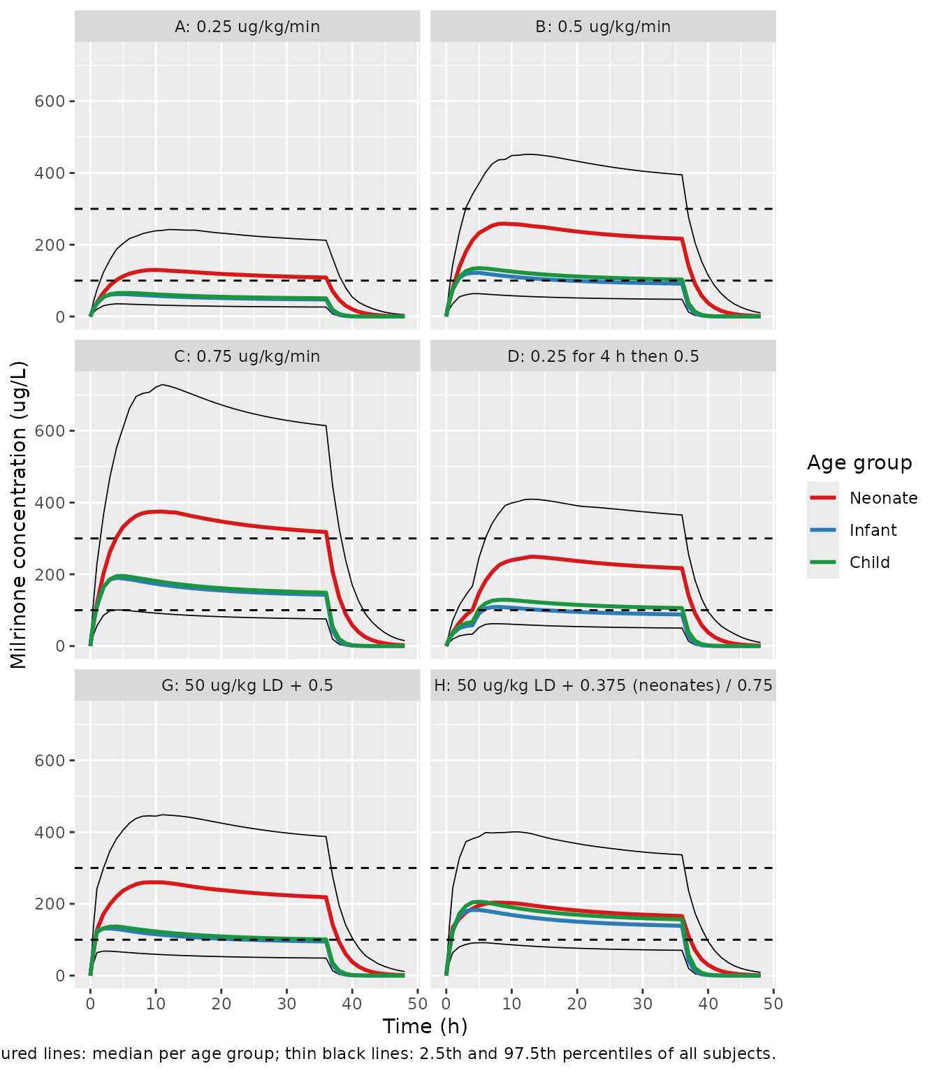
Replicates Figure 3 (panels A-D, G and H) of O’Hanlon 2024.
The medians below are compared with values digitised by the maintainers from Figure 3 (read to about +/- 10 ug/L). Because the simulated cohort only approximates the unpublished GAVamycin covariates, agreement within roughly 25% is the expectation, not exact overlap.
fig3_digitised <- tibble::tribble(
  ~regimen,             ~group,    ~time, ~digitised,
  "A: 0.25 ug/kg/min",  "Neonate",     8,  135,
  "A: 0.25 ug/kg/min",  "Infant",      8,   60,
  "B: 0.5 ug/kg/min",   "Neonate",     8,  275,
  "B: 0.5 ug/kg/min",   "Neonate",    36,  245,
  "B: 0.5 ug/kg/min",   "Infant",      8,  125,
  "B: 0.5 ug/kg/min",   "Child",      36,  100,
  "C: 0.75 ug/kg/min",  "Neonate",     8,  410,
  "C: 0.75 ug/kg/min",  "Neonate",    36,  365,
  "C: 0.75 ug/kg/min",  "Infant",      4,  195,
  "C: 0.75 ug/kg/min",  "Child",      36,  150,
  "H: 50 ug/kg LD + 0.375 (neonates) / 0.75", "Neonate", 8, 215,
  "H: 50 ug/kg LD + 0.375 (neonates) / 0.75", "Infant",  4, 200,
  "H: 50 ug/kg LD + 0.375 (neonates) / 0.75", "Child",  36, 150
)
fig3_cmp <- fig3_digitised |>
  left_join(fig3 |> mutate(group = as.character(group)), by = c("regimen", "group", "time")) |>
  mutate(pct_diff = 100 * (Q50 / digitised - 1))
knitr::kable(
  fig3_cmp |>
    rename(Regimen = regimen, `Age group` = group, `Time (h)` = time,
           `Figure 3 median (ug/L)` = digitised, `Simulated median (ug/L)` = Q50,
           `Difference (%)` = pct_diff),
  digits = 0
)| Regimen | Age group | Time (h) | Figure 3 median (ug/L) | Simulated median (ug/L) | Difference (%) |
|---|---|---|---|---|---|
| A: 0.25 ug/kg/min | Neonate | 8 | 135 | 128 | -5 |
| A: 0.25 ug/kg/min | Infant | 8 | 60 | 60 | -1 |
| B: 0.5 ug/kg/min | Neonate | 8 | 275 | 258 | -6 |
| B: 0.5 ug/kg/min | Neonate | 36 | 245 | 217 | -12 |
| B: 0.5 ug/kg/min | Infant | 8 | 125 | 115 | -8 |
| B: 0.5 ug/kg/min | Child | 36 | 100 | 103 | 3 |
| C: 0.75 ug/kg/min | Neonate | 8 | 410 | 371 | -10 |
| C: 0.75 ug/kg/min | Neonate | 36 | 365 | 318 | -13 |
| C: 0.75 ug/kg/min | Infant | 4 | 195 | 190 | -3 |
| C: 0.75 ug/kg/min | Child | 36 | 150 | 149 | -1 |
| H: 50 ug/kg LD + 0.375 (neonates) / 0.75 | Neonate | 8 | 215 | 203 | -5 |
| H: 50 ug/kg LD + 0.375 (neonates) / 0.75 | Infant | 4 | 200 | 183 | -8 |
| H: 50 ug/kg LD + 0.375 (neonates) / 0.75 | Child | 36 | 150 | 157 | 4 |
Assumptions and deviations
-
Batch-2 proportional error. Table 2 prints 0.332
and the published control stream
$THETAprints 0.322; every other control-stream value equals its Table 2 estimate. The maintainers kept the Table 2 value (0.332). Batch 1 is the default whenever both residual-error indicators are 0, so simulations of new subjects are unaffected. - Size descriptor. The paper’s normal fat mass reduces to fat-free mass because Ffat was fixed to 0 for both CL and V; total body mass therefore does not appear in the packaged model. FFM must come from the neonate-to-adult FFM model the authors used (O’Hanlon et al. 2023); the adult Janmahasatian formula is not appropriate for neonates and infants.
-
Renal function.
RENALFUNC_RELis the paper’s RF = eGFR / nGFR from the Day-1 post-surgical serum creatinine carried forward. FCLR (the fraction of CL explained by RF) was fixed to 1, so RF multiplies all of CL. The authors set RF = 1 for the Paradisis neonates (< 2 days old); do the same for any subject whose renal function is assumed normal for age. -
Clock of the time-varying CL.
tin the model is the time since the first milrinone dose (control streamTIME ; h time since first dose), so an event table must start at the first milrinone dose. In the Starship study milrinone started at the end of bypass, so the curve also describes recovery after cardiopulmonary bypass. -
Postnatal age units. The canonical
PNAcolumn is in months; the model converts to days (PNA * 30.4375) for the birth effect on V, whose half-time is 0.969 days. -
Residual-error indicators. The Starship assay
batches and the Paradisis study each have their own combined error,
selected by
ASSAY_BATCH2(batch 2) andSTUDY_PARADISIS2007. The random effectetaRUVscales both components of the residual SD, as in the control stream. The M3 handling of BLQ samples applies to estimation only. -
Names for the paper’s empirical functions. FCL is
encoded as
cl_exp_fdef, a deficit below the asymptotic CL, solclkeeps the paper’s asymptotic CL of 17.6 L/h; FV and TVOL are encoded asvc_pna_fampandlvc_pna_kdes. The half-times TCL and TVOL enter as rate constants,ln(2) / half-time. The maintainers ratified these names. - Virtual cohort. The GAVamycin database used for Figure 3 is not public. The neonate, infant and child cohorts above use approximate growth curves, FFM fractions of body weight of 0.88, 0.75 and 0.80 (the Starship median FFM/weight ratio was 0.72), and normal renal function. Real post-bypass patients usually have RF below 1, which would raise concentrations.
- Loading-dose timing. The paper does not say whether the maintenance infusion starts with or after the 1-h loading dose; the simulation starts it after. Regimens E and F (Vogt 2014 age-banded doses, Supplementary Table S1) are not replicated.
- Figure 3 percentiles are of individual predictions without residual error; the paper does not say whether its prediction intervals included residual error.