Tacrolimus with posaconazole (Chen 2022) • nlmixr2lib

Model and source

Citation: Chen X, Wang D, Zheng F, Zhu L, Huang Y, Zhu Y, Huang Y, Xu H, Li Z. Effects of posaconazole on tacrolimus population pharmacokinetics and initial dose in children with Crohn’s disease undergoing hematopoietic stem cell transplantation. Front Pharmacol. 2022;13:758524. doi:10.3389/fphar.2022.758524.
Description: One-compartment population PK model with first-order absorption for oral tacrolimus whole-blood concentrations in children with Crohn’s disease undergoing haematopoietic stem cell transplantation at a single centre in China (Chen 2022). The absorption rate constant ka is fixed at 4.48 1/h from the literature. Apparent oral clearance CL/F is allometrically scaled by body weight (fixed exponent 0.75, reference 70 kg) and reduced by 57% with concomitant posaconazole; apparent volume V/F is scaled linearly by body weight (fixed exponent 1). Exponential IIV on CL/F and V/F; combined proportional + additive residual error.
Article: https://doi.org/10.3389/fphar.2022.758524 (open access, PMC9043134)

Chen et al. (2022) fitted a one-compartment model with first-order absorption to routine therapeutic-drug-monitoring trough concentrations of oral tacrolimus in children with Crohn’s disease undergoing haematopoietic stem cell transplantation (HSCT). Body weight (fixed allometric exponents, 70 kg reference) and concomitant posaconazole were retained; posaconazole lowers CL/F to 43% of its value without the azole. Because every sample was a trough, the absorption rate constant was fixed at 4.48 1/h from earlier paediatric tacrolimus models. The paper then used Monte Carlo simulation to recommend weight-banded initial doses with and without posaconazole.

The same group published a structurally identical model for children with chronic granulomatous disease co-treated with voriconazole (Chen_2021a_tacrolimus); its vignette uses the same validation approach.

Population

Fifty-one children (32 boys, 19 girls) treated at the Children’s Hospital of Fudan University between October 2017 and December 2020 contributed 424 whole-blood tacrolimus trough concentrations (about eight per child), measured by the Emit 2000 immunoassay. From Table 1: age median 1.36 (range 0.27-7.58) years and weight median 9.50 (3.70-20.60) kg. Twelve children received posaconazole; glucocorticoids (40/51), omeprazole (41/51) and mycophenolic acid (26/51) were also common but were not retained as covariates. The same information is stored in the model metadata:

str(rxode2::rxode(readModelDb("Chen_2022_tacrolimus"))$population)
#> ℹ parameter labels from comments will be replaced by 'label()'
#> List of 14
#>  $ species         : chr "human"
#>  $ n_subjects      : int 51
#>  $ n_studies       : int 1
#>  $ n_concentrations: int 424
#>  $ age_range       : chr "0.27-7.58 years (median 1.36; mean +/- SD 1.86 +/- 1.38)"
#>  $ weight_range    : chr "3.70-20.60 kg (median 9.50; mean +/- SD 9.85 +/- 3.41)"
#>  $ sex_female_pct  : num 37.3
#>  $ race_ethnicity  : chr "Not reported (single centre in Shanghai, China)"
#>  $ disease_state   : chr "Crohn's disease undergoing haematopoietic stem cell transplantation (HSCT), paediatric"
#>  $ dose_range      : chr "Oral tacrolimus, initial dose 0.33-2 mg/day, then adjusted by TDM. Simulations used 0.1-0.8 mg/kg/day divided into two doses."
#>  $ regions         : chr "China (single centre: Children's Hospital of Fudan University, Shanghai)"
#>  $ co_medication   : chr "Posaconazole 12/51, glucocorticoids 40/51, omeprazole 41/51, mycophenolic acid 26/51 (Table 1)."
#>  $ sampling_design : chr "Retrospective routine TDM, October 2017 - December 2020; 424 whole-blood trough concentrations (about eight per"| __truncated__
#>  $ notes           : chr "32 boys and 19 girls. Estimated in NONMEM 7 by FOCE-I; 1000-replicate bootstrap and pcVPC. All concentrations w"| __truncated__

Source trace

Element	Value	Source
Structure: 1-compartment, first-order absorption and elimination	–	Methods, ‘PPK Model’ (CL/F, V/F, Ka)
`lka`	4.48 1/h (fixed)	Methods ‘PPK Model’; Table 2 (Yang 2015; Wang 2019)
`lcl`	19.8 L/h	Table 2; Results equation 6
`lvc`	11300 L	Table 2 (113 x 10^2 L); Results equation 7
`e_wt_cl`	0.75 (fixed), reference 70 kg	Methods equation 3; Results equation 6
`e_wt_vc`	1 (fixed), reference 70 kg	Methods equation 3; Results equation 7
`e_conmed_posaconazole_cl`	-0.57	Table 2 (theta POS); Results equation 6
Posaconazole form `(1 + theta * POS)`	–	Methods equation 5; Results equation 6
Exponential IIV `P = TV(P) * exp(eta)`	–	Methods equation 1
`etalcl`	0.349^2 = 0.121801	Table 2 (omega CL/F = 0.349, read as SD; see below)
`etalvc`	0.859^2 = 0.737881	Table 2 (omega V/F = 0.859, read as SD; see below)
Residual `O = IP * (1 + eps1) + eps2`	–	Methods equation 2
`propSd`	0.259	Table 2 (sigma1, proportional)
`addSd`	1.353 ng/mL	Table 2 (sigma2, additive)

Figure 3: typical CL/F per kilogram

Figure 3 plots the typical tacrolimus CL/F (L/h/kg) against body weight from 5 to 20 kg, without (a) and with (b) posaconazole. The maintainers digitised the curves at 5, 10, 15 and 20 kg from the pixel centroid of each line. The model’s typical-value cl divided by weight should reproduce them, and the posaconazole curve should be 43% of the other at every weight.

mod <- readModelDb("Chen_2022_tacrolimus")
m0 <- rxode2::zeroRe(mod)
#> ℹ parameter labels from comments will be replaced by 'label()'

# Typical-value solves use the model with its random effects zeroed. With
# several subjects rxode2 warns that there is no omega, which is intended here
# (the eta values, where used, are supplied as data columns).
solve_typical <- function(events, ...) {
  withCallingHandlers(
    rxode2::rxSolve(m0, events = events, returnType = "data.frame", ...),
    warning = function(w) {
      if (grepl("omega", conditionMessage(w))) invokeRestart("muffleWarning")
    }
  )
}

fig3_digitised <- tibble::tribble(
  ~WT, ~CONMED_POSACONAZOLE, ~digitised,
  5,  0, 0.5476,
  10, 0, 0.4604,
  15, 0, 0.4157,
  20, 0, 0.3872,
  5,  1, 0.2351,
  10, 1, 0.1977,
  15, 1, 0.1789,
  20, 1, 0.1662
)

ev3 <- fig3_digitised |>
  mutate(id = row_number(), time = 1, evid = 0L, amt = 0, cmt = "central") |>
  select(id, time, evid, amt, cmt, WT, CONMED_POSACONAZOLE)
sim3 <- solve_typical(ev3, keep = c("WT", "CONMED_POSACONAZOLE"))
#> ℹ omega/sigma items treated as zero: 'etalcl', 'etalvc'
fig3 <- fig3_digitised |>
  left_join(
    sim3 |> transmute(WT, CONMED_POSACONAZOLE, model = cl / WT),
    by = c("WT", "CONMED_POSACONAZOLE")
  ) |>
  mutate(pct_diff = 100 * (model / digitised - 1))

fig3 |>
  mutate(
    Posaconazole = ifelse(CONMED_POSACONAZOLE == 1, "yes", "no"),
    across(c(digitised, model), ~ signif(.x, 3)),
    pct_diff = round(pct_diff, 2)
  ) |>
  select(WT, Posaconazole, digitised, model, pct_diff) |>
  rename(
    "Weight (kg)" = WT,
    "Figure 3 (L/h/kg)" = digitised,
    "Model (L/h/kg)" = model,
    "Difference (%)" = pct_diff
  ) |>
  knitr::kable()

Weight (kg)	Posaconazole	Figure 3 (L/h/kg)	Model (L/h/kg)	Difference (%)
5	no	0.548	0.547	-0.08
10	no	0.460	0.460	-0.07
15	no	0.416	0.416	0.01
20	no	0.387	0.387	-0.08
5	yes	0.235	0.235	0.07
10	yes	0.198	0.198	0.07
15	yes	0.179	0.179	-0.07
20	yes	0.166	0.166	0.10


stopifnot(
  nrow(fig3) == 8L,
  !anyNA(fig3$model),
  # Deterministic typical values against a pixel-centroid digitisation that
  # reads to about 0.0015 L/h/kg (~0.8% on the posaconazole curve). Realised
  # maximum 0.1%. A wrong allometric exponent (1 instead of 0.75) flattens the
  # curve and misses by >30% at 5 or 20 kg; a mis-read theta_POS moves the
  # whole lower curve.
  max(abs(fig3$pct_diff)) < 2
)

wt_grid <- seq(5, 20, by = 0.5)
ev3c <- expand.grid(WT = wt_grid, CONMED_POSACONAZOLE = c(0, 1)) |>
  mutate(id = row_number(), time = 1, evid = 0L, amt = 0, cmt = "central")
curve3 <- solve_typical(ev3c, keep = c("WT", "CONMED_POSACONAZOLE"))
#> ℹ omega/sigma items treated as zero: 'etalcl', 'etalvc'
ggplot() +
  geom_line(
    data = curve3,
    aes(WT, cl / WT, colour = factor(CONMED_POSACONAZOLE))
  ) +
  geom_point(
    data = fig3,
    aes(WT, digitised, colour = factor(CONMED_POSACONAZOLE))
  ) +
  scale_colour_manual(
    values = c("0" = "#1b9e77", "1" = "#d95f02"),
    labels = c("0" = "without posaconazole", "1" = "with posaconazole"),
    name = NULL
  ) +
  scale_y_continuous(limits = c(0, 0.7)) +
  labs(x = "Weight (kg)", y = "CL/F (L/h/kg)") +
  theme_bw()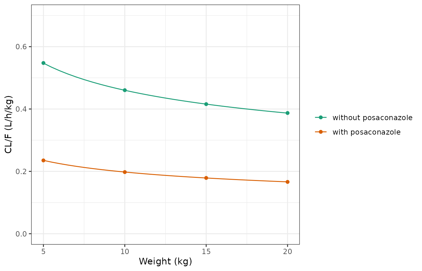

Replicates Figure 3 of Chen 2022: typical CL/F per kilogram against weight. Lines are the model; points are digitised from the figure.

Figures 5 and 6: target attainment and concentration percentiles

Figures 5 (without posaconazole) and 6 (with posaconazole) report, for 1,000 virtual children per scenario, the percentage of simulated tacrolimus concentrations within 5-20 ng/mL (panel A) at body weights of 5, 10, 15 and 20 kg and initial doses of 0.1-0.8 mg/kg/day divided into two doses (every 12 h). Panels B-I show the median and the 5th and 95th percentiles of the simulated concentration for each dose. The maintainers digitised all 64 points of the two panel A plots, and the three percentiles at 5 and 20 kg from panel B (0.1 mg/kg/day) of each figure. Panels C-I are panel B scaled by the dose (their digitised medians at 0.8 mg/kg/day are eight times those at 0.1 mg/kg/day to within 0.5%), so they add no further information.

These figures are also the best evidence for the scale of Table 2’s variability rows. Table 2 prints omega CL/F = 0.349 and omega V/F = 0.859 without saying whether they are standard deviations or variances. The spread of the simulated concentrations depends directly on that choice, so we compute everything under both readings.

The paper calls these “steady-state” concentrations but does not state the sampling time. With V/F = 11300 L at 70 kg the tacrolimus half-life in these children is 10 days or more, so a true steady state would not be reached for weeks. We therefore compute every 12-h trough from 12 h to 120 h and let the figures pick the time, separately for each reading.

To make the result exact and machine-independent, the virtual children are a deterministic 30 x 30 quantile grid of (eta CL/F, eta V/F) passed as data to the model with its random effects zeroed, rather than random draws. The model is linear in dose, so one solve at 0.1 mg/kg/day is scaled to the other seven doses.

pta_digitised <- tibble::tribble(
  ~dose, ~`5`, ~`10`, ~`15`, ~`20`, ~CONMED_POSACONAZOLE,
  0.1, 2.9, 4.4, 5.0, 5.5, 0,
  0.2, 26.1, 28.1, 29.4, 29.2, 0,
  0.3, 46.9, 48.1, 48.2, 48.1, 0,
  0.4, 59.6, 59.1, 59.0, 58.5, 0,
  0.5, 65.7, 66.2, 65.2, 64.8, 0,
  0.6, 67.5, 65.4, 63.9, 63.8, 0,
  0.7, 65.8, 63.3, 62.4, 61.9, 0,
  0.8, 62.8, 61.0, 59.6, 59.8, 0,
  0.1, 8.1, 8.6, 8.7, 8.8, 1,
  0.2, 32.3, 33.1, 33.2, 33.4, 1,
  0.3, 49.2, 49.0, 48.9, 48.9, 1,
  0.4, 57.6, 57.2, 57.5, 57.4, 1,
  0.5, 62.6, 62.3, 61.8, 61.5, 1,
  0.6, 61.1, 60.5, 59.8, 59.7, 1,
  0.7, 59.8, 59.3, 58.6, 58.4, 1,
  0.8, 56.9, 55.9, 55.8, 55.5, 1
) |>
  pivot_longer(c(`5`, `10`, `15`, `20`), names_to = "WT", values_to = "published") |>
  mutate(WT = as.numeric(WT))

# Panel B of each figure: concentrations (ng/mL) at 0.1 mg/kg/day
pct_digitised <- tibble::tribble(
  ~CONMED_POSACONAZOLE, ~WT, ~p05, ~p50, ~p95,
  0, 5,  0.45, 1.60, 4.55,
  0, 20, 0.47, 1.67, 5.05,
  1, 5,  0.45, 1.75, 5.78,
  1, 20, 0.45, 1.78, 6.23
)
stopifnot(nrow(pta_digitised) == 64L, !anyNA(pta_digitised$published))

ng <- 30
zq <- qnorm((seq_len(ng) - 0.5) / ng)
eta_grid <- expand.grid(zc = zq, zv = zq)
trough_times <- seq(12, 120, by = 12)
scenarios <- expand.grid(WT = c(5, 10, 15, 20), CONMED_POSACONAZOLE = c(0, 1))

# "SD" is the eta SD the model file encodes (sqrt of its omega diagonal), so a
# model that encoded the other reading would fail the assertions below.
# "variance" is the rejected alternative: Table 2's printed value (0.349,
# 0.859) taken as a variance, i.e. the square root of the printed value.
omega_model <- rxode2::rxode(mod)$omega
#> ℹ parameter labels from comments will be replaced by 'label()'
sd_encoded <- sqrt(diag(omega_model))[c("etalcl", "etalvc")]
stopifnot(isTRUE(all.equal(unname(sd_encoded), c(0.349, 0.859))))
readings <- list(
  SD = c(cl = unname(sd_encoded[["etalcl"]]), v = unname(sd_encoded[["etalvc"]])),
  variance = sqrt(c(cl = 0.349, v = 0.859))
)

build_grid_events <- function(om, reading, id0) {
  arms <- vector("list", nrow(scenarios))
  for (s in seq_len(nrow(scenarios))) {
    subj <- data.frame(
      id = id0 + (s - 1) * nrow(eta_grid) + seq_len(nrow(eta_grid)),
      WT = scenarios$WT[s],
      CONMED_POSACONAZOLE = scenarios$CONMED_POSACONAZOLE[s],
      etalcl = om[["cl"]] * eta_grid$zc,
      etalvc = om[["v"]] * eta_grid$zv,
      reading = reading
    )
    # 0.1 mg/kg/day divided into two doses every 12 h
    dose <- tidyr::crossing(subj, time = seq(0, max(trough_times) - 12, by = 12)) |>
      mutate(evid = 1L, amt = 0.1 * WT / 2, cmt = "depot")
    obs <- tidyr::crossing(subj, time = trough_times) |>
      mutate(evid = 0L, amt = 0, cmt = "central")
    arms[[s]] <- bind_rows(dose, obs)
  }
  bind_rows(arms)
}

ev56 <- bind_rows(
  build_grid_events(readings$SD, "SD", 0L),
  build_grid_events(readings$variance, "variance", 100000L)
) |>
  arrange(id, time, desc(evid))

sim56 <- solve_typical(ev56, keep = c("WT", "CONMED_POSACONAZOLE", "reading"))
#> ℹ omega/sigma items treated as zero: 'etalcl', 'etalvc'
#> [====|====|====|====|====|====|====|====|====|====] 0:00:06
stopifnot(
  !anyNA(sim56$Cc),
  nrow(sim56) == 2L * nrow(scenarios) * nrow(eta_grid) * length(trough_times)
)

ruv <- rxode2::rxode(mod)$iniDf
#> ℹ parameter labels from comments will be replaced by 'label()'
prop_sd <- ruv$est[ruv$name == "propSd"]
add_sd <- ruv$est[ruv$name == "addSd"]

pta <- sim56 |>
  tidyr::crossing(dose = seq(0.1, 0.8, by = 0.1)) |>
  mutate(
    conc = Cc * dose / 0.1,
    in_ipred = conc >= 5 & conc <= 20,
    res_sd = sqrt(add_sd^2 + (prop_sd * conc)^2),
    in_obs = pnorm(20, conc, res_sd) - pnorm(5, conc, res_sd)
  ) |>
  group_by(reading, time, WT, CONMED_POSACONAZOLE, dose) |>
  summarise(
    pta_ipred = 100 * mean(in_ipred),
    pta_obs = 100 * mean(in_obs),
    .groups = "drop"
  ) |>
  mutate(dose = round(dose, 1))

pct_model <- sim56 |>
  group_by(reading, time, WT, CONMED_POSACONAZOLE) |>
  summarise(
    m05 = unname(quantile(Cc, 0.05)),
    m50 = median(Cc),
    m95 = unname(quantile(Cc, 0.95)),
    .groups = "drop"
  )

scored <- pta |>
  inner_join(pta_digitised, by = c("WT", "CONMED_POSACONAZOLE", "dose")) |>
  group_by(reading, time) |>
  summarise(
    n = n(),
    rmse_ipred = sqrt(mean((pta_ipred - published)^2)),
    rmse_obs = sqrt(mean((pta_obs - published)^2)),
    .groups = "drop"
  ) |>
  inner_join(
    pct_model |>
      inner_join(pct_digitised, by = c("WT", "CONMED_POSACONAZOLE")) |>
      group_by(reading, time) |>
      summarise(
        err_p05 = 100 * max(abs(m05 / p05 - 1)),
        err_p50 = 100 * max(abs(m50 / p50 - 1)),
        err_p95 = 100 * max(abs(m95 / p95 - 1)),
        .groups = "drop"
      ),
    by = c("reading", "time")
  )
stopifnot(all(scored$n == 64L), nrow(scored) == 2L * length(trough_times))

scored |>
  filter(time %in% c(48, 60, 72, 84, 96)) |>
  mutate(across(c(rmse_ipred, rmse_obs, starts_with("err_")), ~ round(.x, 2))) |>
  rename(
    "Omega read as" = reading,
    "Trough time (h)" = time,
    "Panel A RMSE, no residual (points)" = rmse_ipred,
    "Panel A RMSE, with residual (points)" = rmse_obs,
    "Max error 5th pct (%)" = err_p05,
    "Max error median (%)" = err_p50,
    "Max error 95th pct (%)" = err_p95
  ) |>
  knitr::kable()

Omega read as	Trough time (h)	n	Panel A RMSE, no residual (points)	Panel A RMSE, with residual (points)	Max error 5th pct (%)	Max error median (%)	Max error 95th pct (%)
SD	48	64	10.38	10.09	36.92	33.14	27.98
SD	60	64	4.72	5.02	21.42	17.09	14.62
SD	72	64	0.70	2.65	6.03	1.30	4.44
SD	84	64	3.75	4.63	15.91	15.07	17.09
SD	96	64	7.31	7.52	32.27	30.40	29.80
variance	48	64	10.96	10.87	43.47	33.69	22.13
variance	60	64	5.55	6.38	29.55	17.51	9.16
variance	72	64	2.55	4.39	15.72	3.33	10.24
variance	84	64	4.16	5.38	3.81	14.27	23.28
variance	96	64	6.79	7.60	18.49	29.96	36.60


score_at <- function(rd, t, col) {
  v <- scored[[col]][scored$reading == rd & scored$time == t]
  if (length(v) != 1L) stop("no unique score for ", rd, " at ", t, " h")
  v
}
best_time <- scored |>
  group_by(reading) |>
  summarise(t = time[which.min(rmse_ipred)], rmse = min(rmse_ipred), .groups = "drop")
best_time |>
  rename("Omega read as" = reading, "Best trough time (h)" = t, "Panel A RMSE (points)" = rmse) |>
  knitr::kable(digits = 2)

Omega read as	Best trough time (h)	Panel A RMSE (points)
SD	72	0.70
variance	72	2.55


sd_72 <- score_at("SD", 72, "rmse_ipred")
sd_72_obs <- score_at("SD", 72, "rmse_obs")
var_72 <- scored |> filter(reading == "variance", time == 72)

stopifnot(
  # The SD reading, without residual error, at the trough just before the
  # seventh dose (72 h) reproduces all 64 panel A points. The grid is
  # deterministic, so this does not vary between machines. Realised RMSE
  # about 0.7 percentage points, the precision of the digitisation.
  best_time$t[best_time$reading == "SD"] == 72,
  sd_72 < 1.5,
  # ... and the panel B percentiles: realised worst-case errors 1.3%
  # (median), 4.4% (95th) and 6.0% (5th, which is read off a 0-6 ng/mL axis at
  # 0.45 ng/mL, so one pixel is several percent).
  score_at("SD", 72, "err_p50") < 3,
  score_at("SD", 72, "err_p95") < 7,
  score_at("SD", 72, "err_p05") < 10,
  # The variance reading spreads the concentrations too widely: at the same
  # time (also its own best) its panel A RMSE is 2.55 points and its 95th and
  # 5th percentiles miss by 10.2% and 15.7%. Swapping the readings in the
  # model turns these red.
  var_72$rmse_ipred > 1.5,
  var_72$err_p95 > 7,
  var_72$err_p05 > 10,
  # The paper's percentages are of individual predictions: adding the
  # residual error to the SD reading misses by several times as much
  # (realised 2.65 points).
  sd_72_obs > 2 * sd_72
)

The standard-deviation reading, at the trough just before the seventh dose (72 h, after three days of dosing), reproduces both figures: panel A to about 0.7 percentage points over 64 points and the panel B median to within 1.5%. The variance reading, at the same or any other trough time, is worse on every measure, most visibly in the 95th percentile, because its wider spread puts too many children above 20 ng/mL. Adding residual error to the SD reading also misses, so the paper’s figures were computed from individual predictions. The standard-deviation reading is encoded in the model. The Table 2 standard errors point the same way: 15.8% and 14.7% for the two omegas are below sqrt(2/51) = 19.8%, the smallest relative standard error a variance estimated from 51 children can have.

pta72 <- pta |> filter(reading == "SD", time == 72)
ggplot() +
  geom_line(
    data = pta72,
    aes(WT, pta_ipred, colour = factor(dose), group = dose)
  ) +
  geom_point(
    data = pta_digitised,
    aes(WT, published, colour = factor(dose))
  ) +
  facet_wrap(
    ~CONMED_POSACONAZOLE,
    ncol = 1,
    labeller = as_labeller(c(
      "0" = "Figure 5A: without posaconazole",
      "1" = "Figure 6A: with posaconazole"
    ))
  ) +
  labs(
    x = "Weight (kg)",
    y = "Probability within 5-20 ng/mL (%)",
    colour = "Dose (mg/kg/day)"
  ) +
  theme_bw()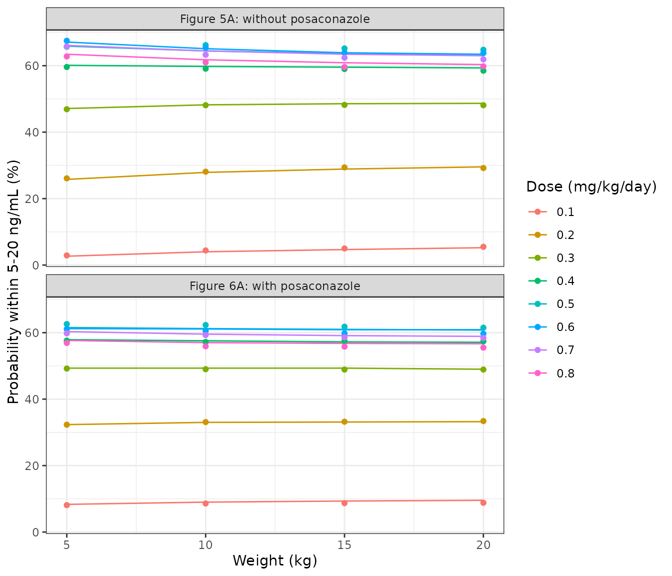

Replicates Figures 5A and 6A of Chen 2022: probability that the 72-h trough is within 5-20 ng/mL without (Figure 5A) and with (Figure 6A) posaconazole. Lines are the model (omega read as SD, no residual error); points are digitised from the figures.

pct72 <- pct_model |>
  filter(reading == "SD", time == 72) |>
  pivot_longer(c(m05, m50, m95), names_to = "stat", values_to = "conc") |>
  mutate(stat = sub("^m", "p", stat))
pct_pts <- pct_digitised |>
  pivot_longer(c(p05, p50, p95), names_to = "stat", values_to = "conc")
ggplot() +
  geom_line(data = pct72, aes(WT, conc, colour = stat)) +
  geom_point(data = pct_pts, aes(WT, conc, colour = stat)) +
  facet_wrap(
    ~CONMED_POSACONAZOLE,
    labeller = as_labeller(c(
      "0" = "Figure 5B: without posaconazole",
      "1" = "Figure 6B: with posaconazole"
    ))
  ) +
  scale_colour_manual(
    values = c(p05 = "#d95f02", p50 = "#1f78b4", p95 = "#33a02c"),
    labels = c(p05 = "5th percentile", p50 = "median", p95 = "95th percentile"),
    name = NULL
  ) +
  labs(x = "Weight (kg)", y = "Tacrolimus (ng/mL)") +
  theme_bw()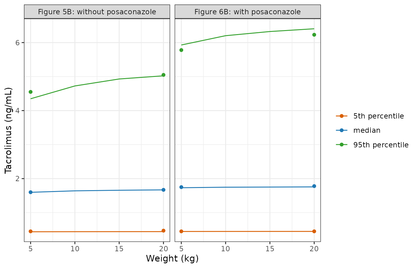

Replicates panel B of Figures 5 and 6 of Chen 2022: median and 5th/95th percentiles of the 72-h trough at 0.1 mg/kg/day. Lines are the model (omega read as SD); points are digitised from the figures.

The paper’s recommendations follow from these figures: without posaconazole, 0.6 mg/kg/day for 5-8.2 kg and 0.5 mg/kg/day for 8.2-20 kg; with posaconazole, 0.5 mg/kg/day for 5-20 kg. At 72 h the concentration is governed mostly by the very large V/F, so the 57% reduction in CL/F changes the median by only about 10% (1.60 against 1.75 ng/mL per 0.1 mg/kg/day at 5 kg); the interaction grows as dosing continues (next section).

Stochastic simulation of the recommended regimens

A 10-kg child (close to the cohort median weight) receives the recommended initial dose of 0.5 mg/kg/day, as two doses 12 h apart, for 28 days, with and without posaconazole. There are 200 virtual children per arm and residual error is included.

nsub <- 200
arms <- tibble::tribble(
  ~arm, ~CONMED_POSACONAZOLE, ~mgkgday,
  "0.5 mg/kg/day, no posaconazole", 0, 0.5,
  "0.5 mg/kg/day, posaconazole", 1, 0.5
)
wt_vpc <- 10
obs_times <- sort(unique(c(seq(0, 672, by = 6), seq(660, 672, by = 1))))
ev_vpc <- bind_rows(lapply(seq_len(nrow(arms)), function(i) {
  ids <- (i - 1) * nsub + seq_len(nsub)
  subj <- data.frame(
    id = ids,
    WT = wt_vpc,
    CONMED_POSACONAZOLE = arms$CONMED_POSACONAZOLE[i],
    arm = arms$arm[i]
  )
  dose <- tidyr::crossing(subj, time = seq(0, 660, by = 12)) |>
    mutate(evid = 1L, amt = arms$mgkgday[i] * wt_vpc / 2, cmt = "depot")
  obs <- tidyr::crossing(subj, time = obs_times) |>
    mutate(evid = 0L, amt = 0, cmt = "central")
  bind_rows(dose, obs)
})) |>
  arrange(id, time, desc(evid))

rxode2::rxSetSeed(2022)
sim_vpc <- rxode2::rxSolve(mod, events = ev_vpc, keep = c("arm"), returnType = "data.frame")
#> ℹ parameter labels from comments will be replaced by 'label()'

vpc_sum <- sim_vpc |>
  group_by(arm, time) |>
  summarise(
    p05 = quantile(sim, 0.05),
    p50 = quantile(sim, 0.5),
    p95 = quantile(sim, 0.95),
    .groups = "drop"
  )

ggplot(vpc_sum, aes(time / 24, p50)) +
  geom_ribbon(aes(ymin = p05, ymax = p95), alpha = 0.25) +
  geom_line() +
  geom_hline(yintercept = c(5, 20), linetype = "dashed") +
  facet_wrap(~arm) +
  labs(
    x = "Time (days)",
    y = "Tacrolimus (ng/mL)",
    caption = "Median and 90% prediction interval, 200 children per arm; dashed lines: 5-20 ng/mL target."
  ) +
  theme_bw()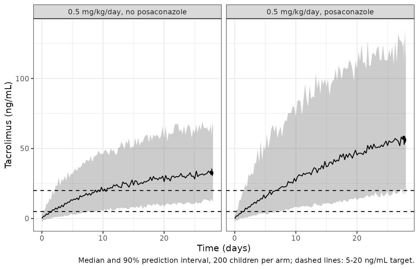

# The model-true median of the 72-h individual prediction comes from the
# deterministic eta grid of the Figures 5 and 6 section (10 kg, omega as SD,
# scaled from 0.1 mg/kg/day to each arm's dose). It is not the typical-value
# prediction: at 72 h the concentration is not log-symmetric in eta V/F.
grid_median <- sim56 |>
  filter(reading == "SD", time == 72, WT == wt_vpc) |>
  group_by(CONMED_POSACONAZOLE) |>
  summarise(grid_med_per_01 = median(Cc), .groups = "drop")
chk <- sim_vpc |>
  filter(time == 72) |>
  group_by(arm) |>
  summarise(median_sim = median(Cc), .groups = "drop") |>
  inner_join(arms, by = "arm") |>
  inner_join(grid_median, by = "CONMED_POSACONAZOLE") |>
  mutate(
    median_grid = grid_med_per_01 * mgkgday / 0.1,
    pct_diff = 100 * (median_sim / median_grid - 1)
  )
chk |>
  select(arm, median_sim, median_grid, pct_diff) |>
  rename(
    "Arm" = arm,
    "Simulated median at 72 h (ng/mL)" = median_sim,
    "Deterministic median at 72 h (ng/mL)" = median_grid,
    "Difference (%)" = pct_diff
  ) |>
  knitr::kable(digits = 2)

Arm	Simulated median at 72 h (ng/mL)	Deterministic median at 72 h (ng/mL)	Difference (%)
0.5 mg/kg/day, no posaconazole	8.64	8.20	5.29
0.5 mg/kg/day, posaconazole	9.57	8.74	9.47

stopifnot(
  nrow(chk) == 2L,
  # 200 children per arm with a log-SD near 0.86 at 72 h give the sample median
  # a standard error of about 8%; 25% is three of them. A dose, unit or volume
  # error moves the median by tens of percent. Realised +5.3% and +9.5%.
  all(abs(chk$pct_diff) < 25)
)

# By day 28 the posaconazole effect on clearance has had time to act: the
# median trough ratio (with / without posaconazole) is well above the 72-h
# ratio of about 1.1. The 1/0.43 = 2.3 clearance ratio is the steady-state limit.
late <- sim_vpc |>
  filter(time == 660) |>
  group_by(arm) |>
  summarise(median_cc = median(Cc), .groups = "drop") |>
  inner_join(arms, by = "arm")
ratio_late <- late$median_cc[late$CONMED_POSACONAZOLE == 1] /
  late$median_cc[late$CONMED_POSACONAZOLE == 0]
ratio_late
#> [1] 1.804809
stopifnot(
  length(ratio_late) == 1L,
  # Realised 1.80 (the typical-value ratio at 660 h is about 1.5; the cohort
  # median sits higher because accumulation is nonlinear in eta). Each sample
  # median carries ~8% error, so the ratio carries ~11%; 1.15 (near the 72-h
  # ratio) is more than three of those below, and 1/0.43 is the steady-state
  # ceiling.
  ratio_late > 1.15,
  ratio_late < 1 / 0.43
)

PKNCA: single-dose typical-value check

The paper reports no non-compartmental results, so there is no published NCA table to compare against. As an internal check, a single 0.2-mg/kg dose to a typical 10-kg child is solved for 8,000 h (more than ten half-lives with posaconazole) and PKNCA’s AUC0-inf should equal Dose/(CL/F).

nca_times <- sort(unique(c(0, 0.05, 0.1, 0.2, 0.3, 0.5, 0.75, 1, 1.5, 2, 3, 4, 6, 8, 12, seq(24, 8000, by = 24))))
ev_nca <- bind_rows(lapply(c(0, 1), function(p) {
  id <- p + 1L
  bind_rows(
    data.frame(id = id, time = 0, evid = 1L, amt = 0.2 * 10, cmt = "depot"),
    data.frame(id = id, time = nca_times, evid = 0L, amt = 0, cmt = "central")
  ) |>
    mutate(
      WT = 10,
      CONMED_POSACONAZOLE = p,
      treatment = ifelse(p == 1, "posaconazole", "no posaconazole")
    )
})) |>
  arrange(id, time, desc(evid))
sim_nca <- solve_typical(ev_nca, keep = c("treatment"), rtol = 1e-10, atol = 1e-12)
#> ℹ omega/sigma items treated as zero: 'etalcl', 'etalvc'
stopifnot(all(sim_nca$Cc >= -1e-6 * max(sim_nca$Cc)))

conc_nca <- sim_nca |>
  filter(!is.na(Cc)) |>
  mutate(Cc = pmax(Cc, 0)) |>
  select(id, time, Cc, treatment)
dose_nca <- ev_nca |>
  filter(evid == 1) |>
  select(id, time, amt, treatment)

o_conc <- PKNCA::PKNCAconc(conc_nca, Cc ~ time | treatment + id)
o_dose <- PKNCA::PKNCAdose(dose_nca, amt ~ time | treatment + id)
o_data <- PKNCA::PKNCAdata(
  o_conc,
  o_dose,
  intervals = data.frame(
    start = 0,
    end = Inf,
    cmax = TRUE,
    tmax = TRUE,
    aucinf.obs = TRUE,
    half.life = TRUE
  )
)
o_nca <- PKNCA::pk.nca(o_data)

nca_wide <- as.data.frame(o_nca$result) |>
  filter(PPTESTCD %in% c("cmax", "tmax", "aucinf.obs", "half.life")) |>
  select(treatment, PPTESTCD, PPORRES) |>
  pivot_wider(names_from = PPTESTCD, values_from = PPORRES)

typ <- sim_nca |>
  distinct(treatment, cl, vc)
nca_chk <- nca_wide |>
  inner_join(typ, by = "treatment") |>
  mutate(
    # dose mg / (L/h) = mg*h/L; x1000 to ng*h/mL
    auc_expected = 1000 * 0.2 * 10 / cl,
    thalf_expected = log(2) * vc / cl,
    auc_pct = 100 * (aucinf.obs / auc_expected - 1),
    thalf_pct = 100 * (half.life / thalf_expected - 1)
  )

nca_chk |>
  select(treatment, cmax, tmax, aucinf.obs, auc_expected, auc_pct, half.life, thalf_expected, thalf_pct) |>
  rename(
    "Treatment" = treatment,
    "Cmax (ng/mL)" = cmax,
    "Tmax (h)" = tmax,
    "AUC0-inf (ng*h/mL)" = aucinf.obs,
    "Dose/(CL/F)" = auc_expected,
    "AUC diff (%)" = auc_pct,
    "t1/2 (h)" = half.life,
    "ln(2)*V/CL (h)" = thalf_expected,
    "t1/2 diff (%)" = thalf_pct
  ) |>
  knitr::kable(digits = 2)

Treatment	Cmax (ng/mL)	Tmax (h)	AUC0-inf (ng*h/mL)	Dose/(CL/F)	AUC diff (%)	t1/2 (h)	ln(2)*V/CL (h)	t1/2 diff (%)
no posaconazole	1.23	1.5	434.69	434.70	0	243.20	243.20	0
posaconazole	1.24	2.0	1010.92	1010.93	0	565.58	565.58	0


stopifnot(
  nrow(nca_chk) == 2L,
  # Deterministic typical-value solve; the trapezoid error on a 24-h grid of a
  # curve with a 240-570 h half-life is well below 1%.
  all(abs(nca_chk$auc_pct) < 1),
  all(abs(nca_chk$thalf_pct) < 1)
)

The half-life is about 240 h without posaconazole and about 570 h with it in a 10-kg child, because V/F is very large relative to CL/F (V/F = 11300 L at 70 kg). This is why the figures’ 72-h trough, three days into dosing, is far from steady state, and why the dose recommendations differ much less between Figures 5 and 6 than the 1:0.43 clearance ratio would suggest.

Assumptions and deviations

Omega scale. Table 2 does not say whether omega CL/F = 0.349 and omega V/F = 0.859 are standard deviations or variances. They are encoded as SDs (variances 0.121801 and 0.737881). Two independent pieces of evidence support this: the standard errors (15.8%, 14.7%) are below the sqrt(2/N) = 19.8% floor for a variance from 51 children, and the SD reading reproduces Figures 5 and 6 (target attainment and percentiles) while the variance reading does not (both asserted above). The same group’s Chen_2021a_tacrolimus model was resolved the same way.
Residual-error scale. sigma1 = 0.259 (proportional) and sigma2 = 1.353 ng/mL (additive) are read as SDs, on the same convention as the omega rows of the same table. Figures 5 and 6 are residual-free and cannot test this. Read as variances they would be SDs of 0.509 and 1.163 ng/mL.
Residual-error form. Methods equation 2, O = IP * (1 + eps1) + eps2 with separate epsilons, is encoded as add(addSd) + prop(propSd), nlmixr2’s default combined form, in which the two variances add.
Figure 5 and 6 sampling time. The paper calls the simulated values steady-state concentrations but does not state when they were taken. The 72-h trough (before the seventh 12-hourly dose) is the best-fitting 12-h trough between 12 and 120 h for the SD reading; with half-lives of 10 days or more, these are not steady-state values. This is a property of the paper’s simulation design, not a model parameter.
Posaconazole indicator. The paper does not report the posaconazole formulation or dose, nor whether POS was allowed to change within a child over time; it is encoded as a per-record covariate so either use is possible.
Screened covariates. Sex, age, the liver and renal laboratory values, the haematology indices and the other co-medications were screened but not retained. They are listed in the model’s covariatesDataExcluded with their Table 1 summaries; the stepwise screening table (Supplementary Table S2) was not needed to build the final model.
Race. The paper does not report race or ethnicity. The children were treated at a single centre in Shanghai, China.
Absorption rate. Ka = 4.48 1/h is fixed from the literature (Yang 2015 and Wang 2019, both paediatric tacrolimus models).
Errata. A Crossref check (2026-10-01) found no correction notice for this article.