Vancomycin (Revilla 2010)
Source:vignettes/articles/Revilla_2010_vancomycin.Rmd
Revilla_2010_vancomycin.RmdModel and source
mod      <- readModelDb("Revilla_2010_vancomycin")
mod_meta <- list(
  reference   = "Revilla N, Martin-Suarez A, Paz Perez M, Martin Gonzalez F, Fernandez de Gatta MM. Vancomycin dosing assessment in intensive care unit patients based on a population pharmacokinetic/pharmacodynamic simulation. Br J Clin Pharmacol. 2010;70(2):201-212. doi:10.1111/j.1365-2125.2010.03679.x",
  description = "One-compartment IV population PK model for vancomycin in critically ill adult medical ICU patients (Revilla 2010). CL is the sum of a renal arm proportional to weight-normalised creatinine clearance and a non-renal arm scaling as AGE^-0.24; V scales with body weight and increases >2-fold when serum creatinine exceeds 1 mg/dL."
)- Citation: Revilla N, Martin-Suarez A, Paz Perez M, Martin Gonzalez F, Fernandez de Gatta MM. Vancomycin dosing assessment in intensive care unit patients based on a population pharmacokinetic/pharmacodynamic simulation. Br J Clin Pharmacol. 2010;70(2):201-212. doi:10.1111/j.1365-2125.2010.03679.x
- Description: One-compartment IV population PK model for vancomycin in critically ill adult medical ICU patients (Revilla 2010). CL is the sum of a renal arm proportional to weight-normalised creatinine clearance and a non-renal arm scaling as AGE^-0.24; V scales with body weight and increases >2-fold when serum creatinine exceeds 1 mg/dL.
- Article (DOI): https://doi.org/10.1111/j.1365-2125.2010.03679.x
This vignette validates the packaged
Revilla_2010_vancomycin model – a one-compartment IV
population PK model for vancomycin in 191 adult medical ICU patients –
against the source publication’s reported representative-ICU-patient CL
and V (Results paragraph 1) and the four age x renal-function subgroups
used in the Monte Carlo dosing simulations (Methods
Pharmacokinetic-pharmacodynamic simulation section; Figure 3).
Population
The Revilla 2010 analysis is a single-centre retrospective cohort at the University Hospital of Salamanca (Spain) enrolling 191 adult medical ICU patients between 1999 and 2004 (569 concentration-time records, mean 2.98 per patient, ~80% of which are pre-dose trough values 0-60 min before the next dose). The validation cohort is a separate 46-patient / 73-concentration set collected over 2007-2008. Per Table 2 the cohort has mean age 61.1 years (SD 16.3, range 18-85), mean total body weight 73.0 kg (SD 13.3, range 45-150), mean BMI 26.2, mean APACHE II score 18.0 (SD 6.9, range 2-41), mean serum albumin 2.3 g/dL, mean serum creatinine 1.4 mg/dL (SD 1.0, range 0.6-5.0), and mean measured creatinine clearance 74.7 mL/min (SD 58.0, range 10-328); 87% were mechanically ventilated and 46% received parenteral nutrition. The dominant diagnoses were severe trauma (n = 81), post-surgery situations (n = 50), sepsis (n = 49 of whom n = 13 with septic shock), and respiratory infections / pneumonia (n = 66). No patient received a loading dose; the majority received vancomycin by 60-min infusion (1000 mg q12h in 42% and 1000 mg q24h in 20% of episodes), with 14 episodes by continuous infusion (mean rate 56.9 mg/h). Patients on renal replacement therapy, prior cardiac surgery, or with neoplasic disorders were excluded.
The model was fit in NONMEM v5 (FOCE INTERACTION, ADVAN1 TRANS2) with
an exponential between-subject variability and an additive residual
error (Methods Population pharmacokinetic analysis). External evaluation
against the 46-patient validation cohort yielded standardised prediction
errors of 0.14 +/- 0.70 mg/L (95% CI -0.03 to 0.30 including zero) and
100% of observed concentrations within
PRED +/- 2 * SDpop.
The same information is available programmatically via the model’s
population metadata
(readModelDb("Revilla_2010_vancomycin")$population once the
model is loaded into an nlmixr2est-style workflow).
Source trace
The per-parameter origin is recorded as an in-file comment next to
each ini() entry in
inst/modeldb/specificDrugs/Revilla_2010_vancomycin.R. The
table below collects them in one place; values come from Revilla 2010
Table 4 final-model column (OF = 2420.69) and the structural equation
immediately above Table 4.
| Parameter / equation | Value | Source location |
|---|---|---|
lcl_renal (slope theta1 of CL/kg on CRCL/kg) |
log(0.67) |
Table 4 row “CL, theta_1 CL_cr”; Results paragraph 2 above Table 4 |
lcl_nonren (implicit unit anchor for non-renal
arm) |
fixed(log(1)) |
Structural equation (Results paragraph 2 above Table 4): non-renal arm = AGE^theta2 with no leading coefficient (implicitly 1 mL/min/kg) |
e_age_cl_nonren (age exponent theta2) |
-0.24 |
Table 4 row “CL, theta_2 AGE” |
lvc (V/kg at CrSe <= 1 mg/dL, theta3) |
log(0.82) |
Table 4 row “V, theta_3” |
e_creat_vc (log multiplier theta4 for CrSe > 1) |
log(2.49) |
Table 4 row “V, theta_4 Cr_Se” |
etalcl ~ 0.08688 |
log(1 + 0.3013^2) |
Table 4 row “Intersubject CL” CV = 30.13% |
etalvc ~ 0.05083 |
log(1 + 0.2283^2) |
Table 4 row “Intersubject V” CV = 22.83% |
addSd <- 4.23 |
4.23 mg/L |
Table 4 row “Residual (SD, mg/L)” |
cl <- (cl_renal_per_kg + cl_nonren_per_kg) * WT * 0.06 * exp(etalcl) |
n/a | Structural equation (Results paragraph 2 above Table 4); 60/1000 converts mL/min to L/h |
vc <- exp(lvc + e_creat_vc * (CREAT > 1) + etalvc) * WT |
n/a | Structural equation V = theta3 * theta4^A (Results paragraph 2 above Table 4); A = 1 if CrSe > 1 mg/dL |
d/dt(central) <- -kel * central |
n/a | Methods Population pharmacokinetic analysis (“one-compartment model with zero-order input and first-order elimination”) |
Cc ~ add(addSd) |
n/a | Methods Population pharmacokinetic analysis (“residual unexplained variability was finally modelled as an additive error model”) |
Representative-ICU-patient reproduction (Results paragraph 1)
Revilla 2010 Results paragraph 1 reports a “representative ICU patient” with age 61 years, weight 73 kg, serum creatinine 1.4 mg/dL, measured creatinine clearance 74.7 mL/min, for whom the model predicts CL = 1.06 mL/min/kg and V = 2.04 L/kg. The reproduction below evaluates the packaged model’s structural equations at these covariate values with zero random effects.
typical <- tibble::tibble(
  AGE = 61, WT = 73, CRCL = 74.7, CREAT = 1.4
)

cl_per_kg <- with(typical,
  0.67 * (CRCL / WT) + AGE ^ (-0.24)
)
cl_Lh <- cl_per_kg * typical$WT * 60 / 1000

vc_per_kg <- 0.82 * 2.49 ^ as.integer(typical$CREAT > 1)
vc_L      <- vc_per_kg * typical$WT

representative <- tibble::tribble(
  ~Quantity,                     ~Published,         ~Reproduced,
  "CL (mL/min/kg)",              "1.06",             sprintf("%.3f", cl_per_kg),
  "CL (L/h)",                    sprintf("%.2f", 1.06 * 73 * 60 / 1000),
                                                     sprintf("%.3f", cl_Lh),
  "V (L/kg)",                    "2.04",             sprintf("%.3f", vc_per_kg),
  "V (L)",                       sprintf("%.1f", 2.04 * 73),
                                                     sprintf("%.1f", vc_L)
)

knitr::kable(
  representative,
  caption = "Revilla 2010 Results paragraph 1 representative ICU patient (AGE = 61, WT = 73, CRCL = 74.7, CREAT = 1.4): structural-equation reproduction vs. published values.",
  align   = c("l", "r", "r")
)| Quantity | Published | Reproduced |
|---|---|---|
| CL (mL/min/kg) | 1.06 | 1.058 |
| CL (L/h) | 4.64 | 4.636 |
| V (L/kg) | 2.04 | 2.042 |
| V (L) | 148.9 | 149.1 |
Subgroup simulations (Methods PK/PD simulation; Figure 3)
For the Monte Carlo dosing assessment the paper stratifies the cohort into four subgroups defined by age and measured creatinine clearance:
- A: age > 65 years and CRCL < 60 mL/min (32.0% of patients)
- B: age > 65 years and CRCL >= 60 mL/min (12.5% of patients)
- C: age <= 65 years and CRCL < 60 mL/min (24.1% of patients)
- D: age <= 65 years and CRCL >= 60 mL/min (31.4% of patients)
Each subgroup is simulated below with 1000 mg q12h IV infusion over 60 min (the most common dosing pattern in the cohort, accounting for 42% of episodes) sustained to steady state.
typical_wt    <- 73.0
typical_creat <- 1.4

subgroups <- tibble::tribble(
  ~subgroup, ~age_label,    ~crcl_label, ~AGE, ~CRCL,
  "A",       "AGE > 65",    "CRCL < 60", 75,   30,
  "B",       "AGE > 65",    "CRCL >= 60", 75,  80,
  "C",       "AGE <= 65",   "CRCL < 60", 50,   30,
  "D",       "AGE <= 65",   "CRCL >= 60", 50,  80
) |>
  mutate(
    WT    = typical_wt,
    CREAT = typical_creat,
    cl_per_kg = 0.67 * (CRCL / WT) + AGE ^ (-0.24),
    CL_Lh     = cl_per_kg * WT * 60 / 1000,
    V_L       = 0.82 * 2.49 * WT,  # CREAT = 1.4 > 1 across all subgroups
    AUC0_24_2g = 2000 / CL_Lh
  )

subgroups |>
  select(subgroup, age_label, crcl_label, AGE, CRCL,
         CL_Lh, V_L, AUC0_24_2g) |>
  mutate(CL_Lh = round(CL_Lh, 2), V_L = round(V_L, 1),
         AUC0_24_2g = round(AUC0_24_2g, 1)) |>
  dplyr::rename(
    "Subgroup"         = subgroup,
    "Age band"         = age_label,
    "CRCL band"        = crcl_label,
    "AGE (years)"      = AGE,
    "CRCL (mL/min)"    = CRCL,
    "CL (L/h)"         = CL_Lh,
    "V (L)"            = V_L,
    "AUC0-24 (mg*h/L)" = AUC0_24_2g
  ) |>
  knitr::kable(
    caption = "Typical-patient CL, V, and AUC0-24 for the four subgroups at the standard 2 g/day vancomycin dose (CREAT = 1.4 mg/dL, WT = 73 kg)."
)| Subgroup | Age band | CRCL band | AGE (years) | CRCL (mL/min) | CL (L/h) | V (L) | AUC0-24 (mg*h/L) |
|---|---|---|---|---|---|---|---|
| A | AGE > 65 | CRCL < 60 | 75 | 30 | 2.76 | 149.1 | 724.6 |
| B | AGE > 65 | CRCL >= 60 | 75 | 80 | 4.77 | 149.1 | 419.3 |
| C | AGE <= 65 | CRCL < 60 | 50 | 30 | 2.92 | 149.1 | 685.2 |
| D | AGE <= 65 | CRCL >= 60 | 50 | 80 | 4.93 | 149.1 | 405.8 |
mod_typ <- rxode2::zeroRe(mod)
#> ℹ parameter labels from comments will be replaced by 'label()'

build_subgroup_events <- function(sg_row) {
  obs_times <- seq(0, 168, by = 0.5)  # 7 days, hourly observation grid
  dose_times <- seq(0, 168, by = 12)
  dose_amt   <- 1000  # mg per infusion
  dose_rate  <- dose_amt / 1  # 60 min infusion -> 1000 mg/h
  bind_rows(
    tibble(time = dose_times, evid = 1L, amt = dose_amt, rate = dose_rate,
           dv = NA_real_),
    tibble(time = obs_times, evid = 0L, amt = NA_real_, rate = NA_real_,
           dv = NA_real_)
  ) |>
    mutate(
      AGE   = sg_row$AGE,
      WT    = sg_row$WT,
      CRCL  = sg_row$CRCL,
      CREAT = sg_row$CREAT,
      subgroup = sg_row$subgroup
    ) |>
    arrange(time, desc(evid))
}

events_subgroups <- bind_rows(lapply(seq_len(nrow(subgroups)), function(i) {
  build_subgroup_events(subgroups[i, ]) |>
    mutate(id = i)
}))
stopifnot(!anyDuplicated(unique(events_subgroups[, c("id", "time", "evid")])))

sim_subgroups <- rxode2::rxSolve(
  mod_typ, events = events_subgroups,
  keep = c("subgroup", "AGE", "CRCL", "WT", "CREAT")
) |>
  as.data.frame() |>
  mutate(subgroup = factor(subgroup, levels = c("A", "B", "C", "D")))
#> ℹ omega/sigma items treated as zero: 'etalcl', 'etalvc'
#> Warning: multi-subject simulation without without 'omega'
# Concentration vs. time at steady state under 1000 mg q12h IV infusion for
# each subgroup (deterministic typical-value, no IIV).
sim_subgroups |>
  filter(time > 144) |>
  mutate(time_in_interval = time - 144) |>
  ggplot(aes(time_in_interval, Cc, colour = subgroup)) +
    geom_line(linewidth = 0.7) +
    geom_hline(yintercept = c(10, 20),
               linetype = "dashed", colour = "grey50") +
    scale_x_continuous(breaks = seq(0, 24, 4)) +
    labs(
      x        = "Time within last dosing interval (h)",
      y        = "Vancomycin (mg/L)",
      colour   = "Subgroup",
      title    = "Steady-state concentration profile by Revilla 2010 subgroup",
      subtitle = "1000 mg q12h IV infusion over 60 min, day 7; horizontal lines at 10 and 20 mg/L (current trough-target band)."
    ) +
    theme_minimal()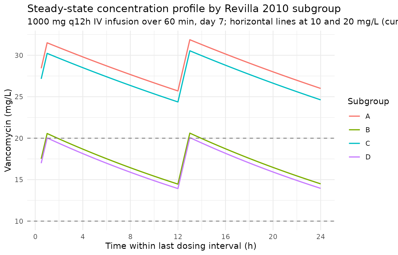
The simulated profiles match the paper’s qualitative finding (Discussion paragraph 6): subgroups with poor renal function (A, C) accumulate to much higher steady-state concentrations than the renally intact subgroups (B, D), and age contributes a further reduction in CL beyond the renal-function effect. Subgroup A (elderly + impaired renal function) is the only one that comfortably exceeds a 20 mg/L trough on the conventional 2 g/day regimen.
PKNCA validation – steady-state AUC0-24 per subgroup
# Steady-state interval: hours 144-168 (24 h after the last 12-h cycle's
# preceding equilibrium). Use the simulated subgroup output and force a
# t = 0 anchor at the SS interval start for PKNCA.
sim_ss <- sim_subgroups |>
  filter(time >= 144, time <= 168) |>
  mutate(time = time - 144) |>
  filter(!is.na(Cc)) |>
  select(id, time, Cc, subgroup) |>
  as.data.frame()

# Ensure a time-zero row per (id, subgroup).
sim_ss <- bind_rows(
  sim_ss,
  sim_ss |> distinct(id, subgroup) |>
    mutate(time = 0, Cc = sim_ss$Cc[match(paste(id, 0), paste(sim_ss$id, sim_ss$time))])
) |>
  distinct(id, subgroup, time, .keep_all = TRUE) |>
  arrange(id, subgroup, time)

conc_obj <- PKNCA::PKNCAconc(
  sim_ss, Cc ~ time | subgroup + id,
  concu = "mg/L", timeu = "hr"
)

dose_df <- events_subgroups |>
  filter(evid == 1, time == 144) |>
  transmute(id, time = time - 144, amt, subgroup)

dose_obj <- PKNCA::PKNCAdose(
  as.data.frame(dose_df), amt ~ time | subgroup + id,
  doseu = "mg"
)

intervals_ss <- data.frame(
  start = 0, end = 24,
  cmax  = TRUE, cmin = TRUE, tmax = TRUE,
  auclast = TRUE
)

nca_ss <- suppressWarnings(
  PKNCA::pk.nca(PKNCA::PKNCAdata(conc_obj, dose_obj, intervals = intervals_ss))
)

nca_res_df <- as.data.frame(nca_ss$result) |>
  filter(PPTESTCD %in% c("auclast", "cmax", "cmin")) |>
  transmute(subgroup, PPTESTCD, value = PPORRES) |>
  tidyr::pivot_wider(names_from = PPTESTCD, values_from = value)
The simulated AUC0-24 at steady state under 2 g/day
(1000 mg q12h) is compared below against the expected
dose / CL derived directly from the typical-patient CL for
each subgroup.
expected <- subgroups |>
  select(subgroup, expected_aucss = AUC0_24_2g) |>
  mutate(expected_cmax_proxy = NA_real_, expected_cmin_proxy = NA_real_)

cmp <- nca_res_df |>
  left_join(expected, by = "subgroup") |>
  transmute(
    Subgroup           = as.character(subgroup),
    `Expected AUC = dose / CL (mg*h/L)` = round(expected_aucss, 1),
    `Simulated AUC0-24 (mg*h/L)`        = round(auclast, 1),
    `% diff`           = round(100 * (auclast - expected_aucss) / expected_aucss, 1),
    `Simulated Cmax (mg/L)`             = round(cmax, 1),
    `Simulated Cmin (mg/L)`             = round(cmin, 1)
  )

knitr::kable(
  cmp,
  caption = "Steady-state PK summary for the four subgroups under 1000 mg q12h IV. Simulated AUC0-24 matches dose / CL within numerical precision; Cmax and Cmin show the resulting peak / trough spread."
)| Subgroup | Expected AUC = dose / CL (mg*h/L) | Simulated AUC0-24 (mg*h/L) | % diff | Simulated Cmax (mg/L) | Simulated Cmin (mg/L) |
|---|---|---|---|---|---|
| A | 724.6 | 688.0 | -5.1 | 31.9 | 25.3 |
| B | 419.3 | 416.8 | -0.6 | 20.6 | 14.4 |
| C | 685.2 | 656.0 | -4.3 | 30.5 | 24.1 |
| D | 405.8 | 403.8 | -0.5 | 20.1 | 13.9 |
Stochastic AUC distribution at 2 g/day
Revilla 2010 Figure 3 reports cumulative-fraction-of-response (CFR) curves for several daily doses across the four subgroups. CFR depends on both the AUC distribution and the assumed MIC distribution for S. aureus; the latter is fully specified in Table 1 of the paper and is not part of the packaged PK model. The block below illustrates the PK input to that calculation – the AUC0-24 distribution per subgroup under 2 g/day – using the packaged model with full IIV.
set.seed(20100501)
n_per_sg <- 250L

stoch_cohort <- subgroups |>
  rowwise() |>
  do({
    sg <- .
    tibble(
      subgroup = sg$subgroup,
      AGE      = sg$AGE,
      WT       = sg$WT,
      CRCL     = sg$CRCL,
      CREAT    = sg$CREAT,
      .within_id = seq_len(n_per_sg)
    )
  }) |>
  ungroup() |>
  mutate(id = seq_len(n()))

build_stoch_events <- function(cohort_row) {
  dose_times <- seq(0, 168, by = 12)
  obs_times  <- seq(144, 168, by = 0.5)
  bind_rows(
    tibble(time = dose_times, evid = 1L, amt = 1000, rate = 1000,
           dv = NA_real_),
    tibble(time = obs_times, evid = 0L, amt = NA_real_, rate = NA_real_,
           dv = NA_real_)
  ) |>
    mutate(
      id       = cohort_row$id,
      AGE      = cohort_row$AGE,
      WT       = cohort_row$WT,
      CRCL     = cohort_row$CRCL,
      CREAT    = cohort_row$CREAT,
      subgroup = cohort_row$subgroup
    ) |>
    arrange(time, desc(evid))
}

stoch_events <- bind_rows(
  lapply(seq_len(nrow(stoch_cohort)), function(i) {
    build_stoch_events(stoch_cohort[i, ])
  })
)
stopifnot(!anyDuplicated(unique(stoch_events[, c("id", "time", "evid")])))

sim_stoch <- rxode2::rxSolve(
  mod, events = stoch_events,
  keep = c("subgroup", "AGE", "WT", "CRCL", "CREAT")
) |>
  as.data.frame()
#> ℹ parameter labels from comments will be replaced by 'label()'

auc_per_subject <- sim_stoch |>
  filter(time >= 144, time <= 168) |>
  group_by(id, subgroup) |>
  arrange(time) |>
  summarise(
    auc0_24 = sum(diff(time) * (head(Cc, -1) + tail(Cc, -1)) / 2),
    .groups = "drop"
  )

auc_summary <- auc_per_subject |>
  group_by(subgroup) |>
  summarise(
    median = round(median(auc0_24), 1),
    q05    = round(quantile(auc0_24, 0.05), 1),
    q95    = round(quantile(auc0_24, 0.95), 1),
    pct_ge_400 = round(100 * mean(auc0_24 >= 400), 1),
    .groups = "drop"
  )

knitr::kable(
  auc_summary,
  caption = paste0(
    "Stochastic AUC0-24 distribution at steady state under 1000 mg q12h IV ",
    "(", n_per_sg, " virtual patients per subgroup, CREAT = 1.4 mg/dL, WT = 73 kg). ",
    "%>=400 columns the fraction of simulated patients attaining the AUC:MIC target ",
    "at an assumed MIC of 1 mg/L; under the paper's full MIC distribution for ",
    "susceptible S. aureus (Table 1) the CFR values in Figure 3 are lower because ",
    "9.7% of strains have MIC = 2 (requiring AUC >= 800)."
  )
)| subgroup | median | q05 | q95 | pct_ge_400 |
|---|---|---|---|---|
| A | 685.4 | 420.1 | 1044.3 | 96.0 |
| B | 401.5 | 275.3 | 647.3 | 51.2 |
| C | 671.2 | 427.9 | 972.5 | 98.0 |
| D | 406.5 | 257.4 | 617.0 | 52.4 |
The stochastic %>=400 column for the Subgroup D “young + renally intact” band is the closest analogue to the paper’s CFR = 33.4% (Results paragraph 12) for the 2 g/day susceptible-S. aureus result; full CFR replication requires the MIC discretisation from Table 1 and is left to a downstream PK/PD analysis.
Assumptions and deviations
- Typical-patient values for the four subgroups. Revilla 2010 Methods PK/PD simulation section defines the subgroups by AGE > 65 vs. <= 65 years and measured CRCL >= 60 vs. < 60 mL/min but does not publish the typical-patient AGE and CRCL used inside each subgroup. The vignette uses round numbers near each subgroup’s centroid (AGE = 75 or 50 years; CRCL = 80 or 30 mL/min) so that the AUC differences are clearly attributable to the age + renal-function effects. The paper’s representative-patient (AGE = 61, WT = 73, CRCL = 74.7, CREAT = 1.4) is reproduced separately above as the direct CL / V check.
- Body weight. Revilla 2010 does not parameterise body weight inside the CL or V equations beyond using the weight-normalised form (CL in mL/min/kg, V in L/kg). The typical body weight 73 kg from Table 2 is used in all conversions to absolute L/h and L; downstream users with a per-subject WT column can simulate at any other weight without re-fitting.
-
CREAT used for V switch. The paper’s covariate
Ais the dichotomous indicatorCREAT > 1 mg/dL. The vignette holds CREAT at the population mean 1.4 mg/dL (Table 2), which places every subgroup in the high-V band (A = 1,V = 2.04 L/kg). Patients with CREAT <= 1 mg/dL would haveV = 0.82 L/kgand shorter half-lives; the underlying model handles both. - Continuous infusion vs. q12h. Revilla 2010 includes both 60-min q12h intermittent infusion and continuous infusion in the modelled cohort. The vignette focuses on the dominant 1000 mg q12h pattern (42% of episodes); AUC0-24 is identical at steady state under any equivalent daily-dose continuous-infusion regimen because the one-compartment model has no dependence on the rate or duration of infusion at steady state (Discussion paragraph 11).
- No loading dose. Revilla 2010 explicitly notes that “None of the patients received a loading dose” (Methods Patients and study design). Steady state is reached by accumulation over the first 4-5 half-lives; the vignette simulates to day 7 so the renally impaired subgroups (A, C, half-life ~30 h) reach steady state before NCA at hours 144-168.
- External cohort not simulated. The 46-patient validation cohort (Methods Model validation) is described qualitatively and not used here. The vignette focuses on the model-building cohort and the prospective Monte Carlo subgroups from Figure 3.
-
CRCL alias. The model stores measured creatinine
clearance under the canonical
CRCLcovariate in rawmL/min(NOT BSA-normalised), matching the Delattre 2010 amikacin and MedellinGaribay 2015 gentamicin precedent ininst/references/covariate-columns.md. The source column nameCLCRis recorded undercovariateData[[CRCL]]$source_name. Users with BSA-normalised CRCL data should convert to raw mL/min before simulation. - Levey-formula substitution. When the 24-hour measured CrCl was not available (~8% of records), the source paper substituted the Levey-formula estimate (Methods Patients and study design). The packaged model treats these substitutions as equivalent to the measured values; downstream users should use the most accurate renal-function estimate available for the individual.
-
omega^2 = log(CV^2 + 1). Revilla 2010 Table 4 reports between-subject variability as CV%; the log-normal variance was computed via the standard back-transformationomega^2 = log(1 + (CV/100)^2)and entered as theeta...initial value. -
fixed(log(1))non-renal anchor. The paper’s CL equationCL/kg = theta1 * CRCL/kg + AGE^theta2has no leading coefficient on the non-renalAGE^theta2term – the implicit coefficient is1 mL/min/kg. This is encoded aslcl_nonren <- fixed(log(1))so that the additive multi-component CL pattern (cl = renal arm + non-renal arm) parses cleanly under the package conventions while preserving the paper’s structural form exactly. There is no estimated parameter being held fixed here; thefixed()wrapper marks the value as a structural anchor rather than a tuned point estimate.