Carvedilol (Honda 2005)
Source:vignettes/articles/Honda_2005_carvedilol.Rmd
Honda_2005_carvedilol.RmdModel and source
- Citation: Honda M, Nozawa T, Igarashi N, Inoue H, Arakawa R, Ogura Y, Okabe H, Taguchi M, Hashimoto Y. Effect of CYP2D6*10 on the pharmacokinetics of R- and S-carvedilol in healthy Japanese volunteers. Biol Pharm Bull. 2005;28(8):1476-1479. doi:10.1248/bpb.28.1476
- Description: One-compartment population PK model for orally administered racemic carvedilol in 23 healthy Japanese volunteers, with R- and S-enantiomer whole-blood concentrations measured by chiral HPLC at 2 h and 6 h after a single 5- or 10-mg oral dose (Honda 2005). NONMEM ADVAN1/TRANS2 with very rapid absorption: the racemic dose is split equally between two parallel central compartments (central_r, central_s) with no separate absorption depot. CL/F and V/F scale linearly with body weight; an S/R ratio theta_3 (CL/F) and theta_4 (V/F) parameterise the stereoselective difference. One subject-level eta on CL/F and one on V/F are shared between enantiomers (correlated block IIV, rho ~ 0.90). Power-variance residual error with fixed exponent 1/2 (Honda Eq. 3), shared between R- and S-enantiomer observations. CYP2D610 genotype is not in the structural model; Honda 2005 reports the 10-carrier effect only as a post-hoc stratification of the individual Bayes estimates (Figs. 3-4).
- Article: https://doi.org/10.1248/bpb.28.1476
Population
Honda 2005 enrolled 23 healthy Japanese adult volunteers (19 men, 4 women; 22-44 years old, mean 29.1; body weight 47-86 kg, mean 64.7). All participants were physicians or pharmacists at Toyama Medical and Pharmaceutical University and chose their own dose level: nine subjects took 5 mg (two 2.5-mg tablets; mean weight 57.9 +/- 6.7 kg) and fourteen took 10 mg (one 10-mg tablet; mean weight 69.1 +/- 9.9 kg). Carvedilol was administered as the commercial racemic Artist tablet with a glass of water, at least 2 h before a meal, after an overnight fast. Two whole-blood samples were drawn at 2 h and 6 h after dosing and assayed for R- and S-carvedilol separately by chiral HPLC (Methods ‘Assay of Carvedilol’).
CYP2D6 alleles *1, *10, and
*14 were determined by PCR-RFLP, *2 by
allele-specific PCR, and *5 by long-PCR. No *5
or *14 null alleles were detected in the cohort. The
genotype distribution was: 5 *1/*1, 1 *1/*2,
12 *1/*10, 3 *2/*10, 2 *10/*10
–17 of 23 subjects carried at least one *10 allele. The
same demographics are available programmatically via
readModelDb("Honda_2005_carvedilol")$population.
Source trace
Per-parameter origin is recorded as an in-file comment next to each
ini() entry in
inst/modeldb/specificDrugs/Honda_2005_carvedilol.R. The
table below collects them in one place for review.
| Equation / parameter | Value | Source location |
|---|---|---|
lclf = log(theta_1) |
log(1.01 L/h/kg) | Table 1, theta_1 = 1.01 (95% CI 0.84-1.18) |
lvf = log(theta_2) |
log(2.53 L/kg) | Table 1, theta_2 = 2.53 (95% CI 2.04-3.02) |
lratiocl = log(theta_3) |
log(2.13) | Table 1, theta_3 = 2.13 (95% CI 1.64-2.62) |
lratiov = log(theta_4) |
log(2.94) | Table 1, theta_4 = 2.94 (95% CI 1.98-3.90) |
etalclf + etalvf ~ c(0.130, 0.130, 0.161) |
block IIV (lower triangle) | Table 1: omega^2(CL/F) = 0.130; omega^2(V/F) = 0.161; omega(CL/F,V/F) = 0.130 |
propSd_r, propSd_s
|
sqrt(0.0584) = 0.2417 | Table 1, sigma^2 = 0.0584 (95% CI 0.0074-0.1094) shared between R and S |
powExp_r, powExp_s
|
fixed(0.5) | Eq. 3 (Cb^(1/2)) |
| Eq. 1 (CL/F structural) | CL/F_i = theta_1 * theta_3^S * WT * (1 + eta) | Eq. 1, page 1477 |
| Eq. 2 (V/F structural) | V/F_i = theta_2 * theta_4^S * WT * (1 + eta) | Eq. 2, page 1477 |
| Eq. 3 (residual error) | Cb = Cb* + Cb^(1/2) eps | Eq. 3, page 1477 |
ODE for central_r / central_s
|
one-compartment bolus, no depot (“very rapid absorption”) | Methods ‘Estimation of Pharmacokinetic Parameters of Carvedilol’ (NONMEM ADVAN1/TRANS2) |
Virtual cohort
Honda’s individual-level demographics (age, weight, sex, CYP2D6 genotype per subject) are not tabulated in the paper; only the group means and ranges are published. The cohort below reconstructs the aggregate covariate distribution Honda reports –n = 23, dose mix 9 / 14, weight 47-86 kg with group-specific means –and assigns each subject a self-chosen 5 mg or 10 mg dose drawn so the dose / weight strata match Methods ‘Subjects and Study Protocols’.
set.seed(20251029)

n_5mg  <- 9L
n_10mg <- 14L

# Body weight, sampled per subject from a truncated normal anchored on the
# Honda group means (5-mg: 57.9 +/- 6.7 kg, 10-mg: 69.1 +/- 9.9 kg) and
# clipped to the published cohort range 47-86 kg.
rtnorm <- function(n, mean, sd, lo, hi) {
  out <- numeric(n)
  i <- 0L
  while (i < n) {
    cand <- stats::rnorm(1, mean, sd)
    if (cand >= lo && cand <= hi) {
      i <- i + 1L
      out[i] <- cand
    }
  }
  out
}
wt_5mg  <- rtnorm(n_5mg,  mean = 57.9, sd = 6.7, lo = 47, hi = 86)
wt_10mg <- rtnorm(n_10mg, mean = 69.1, sd = 9.9, lo = 47, hi = 86)

cohort <- dplyr::bind_rows(
  tibble::tibble(id = seq_len(n_5mg),                       dose_mg = 5,  WT = wt_5mg),
  tibble::tibble(id = n_5mg + seq_len(n_10mg),              dose_mg = 10, WT = wt_10mg)
)
cohort$treatment <- paste0(cohort$dose_mg, " mg")
knitr::kable(
  cohort %>% group_by(treatment) %>%
    summarise(n = dplyr::n(),
              wt_mean = round(mean(WT), 1),
              wt_sd   = round(stats::sd(WT), 1),
              .groups = "drop"),
  caption = "Virtual cohort summary by dose group."
)| treatment | n | wt_mean | wt_sd |
|---|---|---|---|
| 10 mg | 14 | 67.4 | 7.6 |
| 5 mg | 9 | 59.1 | 5.6 |
A racemic carvedilol dose is delivered as two simultaneous bolus
events: half the dose to central_r and half to
central_s. The observation grid covers 0 to 8 h at 0.25-h
resolution; the published sampling time-points 2 h and 6 h are
highlighted in the figures below.
obs_times <- seq(0, 8, by = 0.25)

build_events <- function(cohort_df) {
  dose_rows <- dplyr::bind_rows(
    cohort_df %>% transmute(id, time = 0, evid = 1L,
                            amt = dose_mg / 2, cmt = "central_r",
                            treatment, WT),
    cohort_df %>% transmute(id, time = 0, evid = 1L,
                            amt = dose_mg / 2, cmt = "central_s",
                            treatment, WT)
  )
  # One observation row per time per subject is enough: rxSolve evaluates
  # every output (both Cc_r and Cc_s) at each observation time regardless
  # of which cmt is listed on the row. Carrying two parallel obs rows
  # would create per-time duplicates that PKNCA rejects.
  obs_rows <- cohort_df[rep(seq_len(nrow(cohort_df)), each = length(obs_times)), ] %>%
    transmute(id, time = rep(obs_times, nrow(cohort_df)), evid = 0L,
              amt = 0, cmt = "Cc_r", treatment, WT)
  dplyr::bind_rows(dose_rows, obs_rows) %>%
    dplyr::arrange(id, time, dplyr::desc(evid))
}

events <- build_events(cohort)
Simulation
mod <- readModelDb("Honda_2005_carvedilol")Typical-value (no random effects) simulation for comparison with the Honda mean trajectories:
mod_typical <- rxode2::zeroRe(mod)
sim_typical <- rxode2::rxSolve(
  mod_typical,
  events = events,
  keep = c("treatment", "WT"),
  returnType = "data.frame"
)
#> ℹ omega/sigma items treated as zero: 'etalclf', 'etalvf'
#> Warning: multi-subject simulation without without 'omega'
Stochastic simulation with the published block-IIV and the power-variance residual error:
Replicate published figures
Honda Figure 1 shows the individual R- and S-carvedilol whole-blood concentrations at 2 h and 6 h for all 23 subjects, with separate panels for the 5-mg and 10-mg dose groups. The simulated typical trajectories below pass through the centre of the published concentration ranges (roughly 0.5-5 ng/mL for R at 2 h and 0.1-2 ng/mL for R at 6 h).
# Replicates Figure 1 of Honda 2005: R- and S-carvedilol blood
# concentrations versus time, by dose group.
plot_df <- sim_typical %>%
  dplyr::filter(time > 0) %>%
  tidyr::pivot_longer(
    cols      = c("Cc_r", "Cc_s"),
    names_to  = "enantiomer",
    values_to = "Cc"
  ) %>%
  dplyr::mutate(enantiomer = dplyr::recode(enantiomer,
                                           "Cc_r" = "R-carvedilol",
                                           "Cc_s" = "S-carvedilol"))

ggplot(plot_df, aes(time, Cc, group = id, colour = treatment)) +
  geom_line(alpha = 0.6) +
  facet_grid(enantiomer ~ treatment) +
  scale_y_log10(limits = c(0.05, 30)) +
  geom_vline(xintercept = c(2, 6), linetype = "dashed", colour = "grey50") +
  labs(x = "Time (h)", y = "Blood concentration (ng/mL)",
       title = "Figure 1 (replicate) -- Typical R- and S-carvedilol profiles",
       caption = "Vertical dashed lines mark the Honda 2005 sampling time-points (2 h and 6 h).")
#> Warning: Removed 2 rows containing missing values or values outside the scale range
#> (`geom_line()`).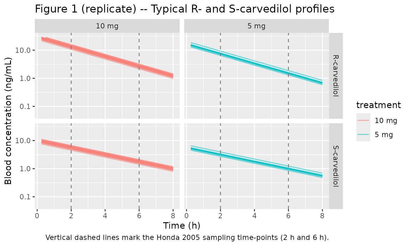
A stochastic VPC using the block-IIV and power-variance residual error captures the scatter across subjects.
# rxSolve returns Cc_r and Cc_s as per-individual predictions when the
# model is solved with active random effects; the same column names are
# reused for typical-value and stochastic sims. Percentiles across the
# 23 simulated subjects mimic a VPC envelope.
vpc_df <- sim_stoch %>%
  dplyr::filter(time > 0) %>%
  tidyr::pivot_longer(
    cols      = c("Cc_r", "Cc_s"),
    names_to  = "enantiomer",
    values_to = "Cc"
  ) %>%
  dplyr::mutate(enantiomer = dplyr::recode(enantiomer,
                                           "Cc_r" = "R-carvedilol",
                                           "Cc_s" = "S-carvedilol")) %>%
  dplyr::group_by(time, treatment, enantiomer) %>%
  dplyr::summarise(Q05 = stats::quantile(Cc, 0.05, na.rm = TRUE),
                   Q50 = stats::quantile(Cc, 0.50, na.rm = TRUE),
                   Q95 = stats::quantile(Cc, 0.95, na.rm = TRUE),
                   .groups = "drop")

ggplot(vpc_df, aes(time, Q50, fill = treatment)) +
  geom_ribbon(aes(ymin = Q05, ymax = Q95), alpha = 0.30) +
  geom_line() +
  facet_grid(enantiomer ~ treatment) +
  scale_y_log10(limits = c(0.05, 50)) +
  labs(x = "Time (h)", y = "Individual-predicted Cc (ng/mL)",
       title = "VPC -- 5th, 50th, 95th percentile of individual predictions",
       caption = "Block-IIV (rho = 0.90) shared between enantiomers per Honda Eq. 1-2.")
#> Warning: Removed 2 rows containing missing values or values outside the scale range
#> (`geom_ribbon()`).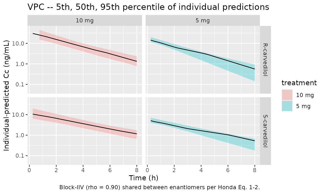
PKNCA validation
Honda 2005 does not tabulate Cmax / Tmax / AUC, but for a
one-compartment bolus model the model-predicted typical AUC follows
Dose / CL. The NCA output below derives Cmax, AUCinf, and
half-life on the dense typical-value profiles; the implied typical CL/F
= Dose / AUCinf provides a direct check against Honda’s
reported theta_1 * WT (R) and
theta_1 * theta_3 * WT (S).
sim_r <- sim_typical %>%
  dplyr::filter(time >= 0) %>%
  dplyr::select(id, time, Cc = Cc_r, treatment) %>%
  dplyr::filter(!is.na(Cc))

dose_r <- events %>%
  dplyr::filter(evid == 1, cmt == "central_r") %>%
  dplyr::select(id, time, amt, treatment)

conc_obj_r <- PKNCA::PKNCAconc(sim_r, Cc ~ time | treatment + id,
                               concu = "ng/mL", timeu = "h")
dose_obj_r <- PKNCA::PKNCAdose(dose_r, amt ~ time | treatment + id,
                               doseu = "mg")

intervals <- data.frame(start = 0, end = Inf,
                        cmax = TRUE, tmax = TRUE,
                        aucinf.obs = TRUE, half.life = TRUE)

nca_data_r <- PKNCA::PKNCAdata(conc_obj_r, dose_obj_r, intervals = intervals)
nca_res_r  <- PKNCA::pk.nca(nca_data_r)
nca_summary_r <- summary(nca_res_r)
knitr::kable(nca_summary_r, caption = "R-carvedilol NCA on typical profiles.")| Interval Start | Interval End | treatment | N | Cmax (ng/mL) | Tmax (h) | Half-life (h) | AUCinf,obs (h*ng/mL) |
|---|---|---|---|---|---|---|---|
| 0 | Inf | 10 mg | 14 | 29.5 [11.1] | 0.000 [0.000, 0.000] | 1.74 [0.000] | 73.9 [11.1] |
| 0 | Inf | 5 mg | 9 | 16.8 [9.79] | 0.000 [0.000, 0.000] | 1.74 [4.84e-16] | 42.0 [9.79] |
sim_s <- sim_typical %>%
  dplyr::filter(time >= 0) %>%
  dplyr::select(id, time, Cc = Cc_s, treatment) %>%
  dplyr::filter(!is.na(Cc))

dose_s <- events %>%
  dplyr::filter(evid == 1, cmt == "central_s") %>%
  dplyr::select(id, time, amt, treatment)

conc_obj_s <- PKNCA::PKNCAconc(sim_s, Cc ~ time | treatment + id,
                               concu = "ng/mL", timeu = "h")
dose_obj_s <- PKNCA::PKNCAdose(dose_s, amt ~ time | treatment + id,
                               doseu = "mg")

nca_data_s <- PKNCA::PKNCAdata(conc_obj_s, dose_obj_s, intervals = intervals)
nca_res_s  <- PKNCA::pk.nca(nca_data_s)
nca_summary_s <- summary(nca_res_s)
knitr::kable(nca_summary_s, caption = "S-carvedilol NCA on typical profiles.")| Interval Start | Interval End | treatment | N | Cmax (ng/mL) | Tmax (h) | Half-life (h) | AUCinf,obs (h*ng/mL) |
|---|---|---|---|---|---|---|---|
| 0 | Inf | 10 mg | 14 | 10.0 [11.1] | 0.000 [0.000, 0.000] | 2.40 [2.46e-16] | 34.7 [11.1] |
| 0 | Inf | 5 mg | 9 | 5.71 [9.79] | 0.000 [0.000, 0.000] | 2.40 [1.57e-16] | 19.7 [9.79] |
Comparison against published parameters
auc_r <- as.data.frame(nca_res_r$result) %>%
  dplyr::filter(PPTESTCD == "aucinf.obs") %>%
  dplyr::transmute(id, treatment, AUCinf_r = PPORRES)
auc_s <- as.data.frame(nca_res_s$result) %>%
  dplyr::filter(PPTESTCD == "aucinf.obs") %>%
  dplyr::transmute(id, AUCinf_s = PPORRES)

dose_per_subj <- events %>% dplyr::filter(evid == 1, cmt == "central_r") %>%
  dplyr::select(id, dose_r = amt)
wt_per_subj <- cohort %>% dplyr::select(id, WT)

implied <- auc_r %>%
  dplyr::left_join(auc_s, by = "id") %>%
  dplyr::left_join(dose_per_subj, by = "id") %>%
  dplyr::left_join(wt_per_subj, by = "id") %>%
  dplyr::mutate(
    # AUCinf is in (ng/mL) * h = ug/L * h; convert to mg/L * h by /1000
    AUCinf_r_mgLh = AUCinf_r / 1000,
    AUCinf_s_mgLh = AUCinf_s / 1000,
    CLF_r_Lhkg = dose_r / (AUCinf_r_mgLh * WT),
    CLF_s_Lhkg = dose_r / (AUCinf_s_mgLh * WT)
  )

compare_tbl <- implied %>%
  dplyr::summarise(
    `Honda theta_1 (L/h/kg)`            = 1.01,
    `Implied typical CL/F_R (L/h/kg)`   = round(mean(CLF_r_Lhkg), 3),
    `Honda theta_1*theta_3 (L/h/kg)`    = 1.01 * 2.13,
    `Implied typical CL/F_S (L/h/kg)`   = round(mean(CLF_s_Lhkg), 3),
    `S/R clearance ratio (implied)`     = round(mean(CLF_s_Lhkg / CLF_r_Lhkg), 3),
    `Honda theta_3`                     = 2.13
  )
knitr::kable(compare_tbl,
caption = "Implied typical CL/F values from NCA vs Honda 2005 Table 1.")| Honda theta_1 (L/h/kg) | Implied typical CL/F_R (L/h/kg) | Honda theta_1*theta_3 (L/h/kg) | Implied typical CL/F_S (L/h/kg) | S/R clearance ratio (implied) | Honda theta_3 |
|---|---|---|---|---|---|
| 1.01 | 1.01 | 2.1513 | 2.151 | 2.13 | 2.13 |
hl_r <- as.data.frame(nca_res_r$result) %>%
  dplyr::filter(PPTESTCD == "half.life") %>%
  dplyr::summarise(median_t12_r_h = stats::median(PPORRES))
hl_s <- as.data.frame(nca_res_s$result) %>%
  dplyr::filter(PPTESTCD == "half.life") %>%
  dplyr::summarise(median_t12_s_h = stats::median(PPORRES))

# Implied typical half-lives from the parameter point estimates
typ_t12_r <- log(2) / (1.01 / 2.53)
typ_t12_s <- log(2) / ((1.01 * 2.13) / (2.53 * 2.94))

tibble::tibble(
  `Half-life`                   = c("R-carvedilol", "S-carvedilol"),
  `Implied from theta values (h)` = c(round(typ_t12_r, 2), round(typ_t12_s, 2)),
  `NCA median (h)`              = c(round(hl_r$median_t12_r_h, 2),
                                    round(hl_s$median_t12_s_h, 2))
) %>%
knitr::kable(caption = "Half-life agreement: parameter-implied vs NCA-derived.")| Half-life | Implied from theta values (h) | NCA median (h) |
|---|---|---|
| R-carvedilol | 1.74 | 1.74 |
| S-carvedilol | 2.40 | 2.40 |
Assumptions and deviations
-
IIV form. Honda Eq. 1 and Eq. 2 use a literal
linear
(1 + eta)parameterisation for inter-individual variability on untransformed CL/F and V/F. The packaged model uses the nlmixr2-standard log-normalexp(lparam + etalparam)form as a close approximation. For Honda’s reported variances (omega^2 = 0.130 and 0.161, CV ~ 36 % and ~ 40 %), the two forms agree to within a few percent on the bulk of the per-subject CL/F distribution but the log-normal form avoids unphysical negative CL/F in the extreme tail ofeta. -
Mu-reference encoding. The S/R ratios
lratiocl(theta_3) andlratiov(theta_4) appear outside theexp(lparam + etalparam)block so nlmixr2’s mu-reference parser sees a single fixed-effect parameter per eta-bearing exponential. The mathematics is unchanged:exp(lclf + etalclf) * exp(lratiocl) * WTequals Honda’stheta_1 * theta_3 * WT * (1 + eta)to log-normal-vs-linear precision. -
Shared sigma. Honda fits one residual-error sigma
shared between R and S observations (single
$SIGMAblock in NONMEM). nlmixr2 requires a distinct residual SD parameter per~endpoint, so the model file declarespropSd_randpropSd_sseparately, both initialised tosqrt(0.0584)and held equal. Users who re-fit the model with both enantiomers simultaneously must constrainpropSd_r = propSd_sto preserve Honda’s structural shared-sigma assumption. -
Fixed power exponent. The power-variance exponent
(Honda Eq. 3,
Cb*^(1/2)) is treated as a fixed structural assumption rather than an estimated parameter, matching the published equation. A future model development that estimates the exponent (analogous to Tod 1998 amikacin’s Power-b) would change this. -
Concentration units and the 1000 factor. Honda
reports whole-blood concentrations in ng/mL but the structural CL/F and
V/F are in L/h/kg and L/kg with dosing in mg. The model multiplies
central / Vby 1000 to convert mg/L to ng/mL so the residual-error sigma is interpreted on the published ng/mL scale. -
Dosing encoding. The racemic carvedilol dose is
delivered to the model as two synchronous bolus events, half the dose
into
central_rand half intocentral_s(no interconversion). Honda’s NONMEM ADVAN1/TRANS2 with “very rapid absorption” is encoded as instantaneous delivery into the central compartment; no depot is carried. -
CYP2D6 not a structural covariate. Honda 2005
reports a significant reduction in (CL/F)/WT and (V/F)/WT in CYP2D6
*10-allele carriers vs. the*1/*1and*1/*2reference complement (Figs. 3-4; p < 0.001 for R-carvedilol CL/F), but the effect is shown only as a t-test on the individual Bayes estimates and the NONMEM structural model does not include CYP2D6 as a covariate. The packaged model therefore does NOT carry a CYP2D6 effect; downstream users who want the*10-carrier stratification can post-process Bayes-estimate output or re-fit with CYP2D6 as a covariate. CYP2D6_PM is documented incovariatesDataExcludedso the paper’s stratification is discoverable. - Sparse Honda sampling, dense simulation. Honda’s two-time-point (2 h and 6 h) sampling was used for Bayesian individual estimation only. The vignette simulates dense profiles purely to drive PKNCA; the resulting NCA Cmax and Tmax values are model-implied rather than comparable to any published observation.