Model and source
- Citation: Lin J, Gaudreault F, Johnson N, Lin Z, Nouri P, Goosen TC, Sawant-Basak A. (2022). Investigation of CYP3A induction by PF-05251749 in early clinical development: comparison of linear slope physiologically based pharmacokinetic prediction and biomarker response. Clin Transl Sci 15(9):2184-2194. doi:10.1111/cts.13352.
- 400 mg model: Two-compartment oral pharmacokinetic reduction of the Simcyp minimal-PBPK-with-single-adjusting-compartment (SAC) base model for the casein kinase 1 delta/epsilon inhibitor PF-05251749 at 400 mg q.d. in healthy adults (Lin 2022). The authors built separate dose-specific Simcyp models at 400 and 750 mg q.d. because exposure was less than dose-proportional above 200 mg; this file is the 400 mg model and Lin_2022_PF05251749_750mg is its sibling. The Simcyp whole-body equations are not published, but the compound layer (Table 2: ka, fa, fu, B:P, observed oral clearance CLpo, Vss, Vsac and the SAC inter-compartmental clearance Q) is enough to rebuild the disposition as first-order absorption into a systemic compartment exchanging with the SAC (peripheral1). Systemic clearance and bioavailability follow from CLpo through the well-stirred liver model; the systemic volume is (Vss - Vsac) x 70 kg minus a liver volume. Hepatic blood flow (90 L/h) and liver volume (1.648 L) are not printed in the paper and are standard Simcyp healthy-adult values. Nothing is fitted. The reduction reproduces the paper’s predicted day-14 Tmax to within 3% and gives AUCtau 7% and Cmax 12% below the paper’s geometric-mean predictions (see the validation vignette). Typical-value model: the source reports no variance components and no residual-error model, so there are no etas and propSd is zero. The CYP3A-induction (midazolam DDI) layer depends on the proprietary Simcyp midazolam compound file and enzyme-turnover defaults and is not encoded.
- 750 mg model: Two-compartment oral pharmacokinetic reduction of the Simcyp minimal-PBPK-with-single-adjusting-compartment (SAC) base model for the casein kinase 1 delta/epsilon inhibitor PF-05251749 at 750 mg q.d. in healthy adults (Lin 2022). The authors built separate dose-specific Simcyp models at 400 and 750 mg q.d. because exposure was less than dose-proportional above 200 mg; this file is the 750 mg model and Lin_2022_PF05251749_400mg is its sibling. The Simcyp whole-body equations are not published, but the compound layer (Table 2: ka, fa, fu, B:P, observed oral clearance CLpo, Vss, Vsac and the SAC inter-compartmental clearance Q) is enough to rebuild the disposition as first-order absorption into a systemic compartment exchanging with the SAC (peripheral1). Systemic clearance and bioavailability follow from CLpo through the well-stirred liver model; the systemic volume is (Vss - Vsac) x 70 kg minus a liver volume. Hepatic blood flow (90 L/h) and liver volume (1.648 L) are not printed in the paper and are standard Simcyp healthy-adult values. Nothing is fitted. The reduction reproduces the paper’s predicted day-14 Tmax to within 3% and gives Cmax and AUCtau 7% below the paper’s geometric-mean predictions (see the validation vignette). Typical-value model: the source reports no variance components and no residual-error model, so there are no etas and propSd is zero. The CYP3A-induction (midazolam DDI) layer depends on the proprietary Simcyp midazolam compound file and enzyme-turnover defaults and is not encoded.
- Article: https://doi.org/10.1111/cts.13352
- Supplement (Tables S1-S5, Figures S1-S5): https://www.ncbi.nlm.nih.gov/pmc/articles/PMC9468555/
What these models are, and what they are not
PF-05251749 is a dual casein kinase 1 delta/epsilon inhibitor that was developed for disrupted circadian rhythm in Alzheimer’s and Parkinson’s disease. It induced CYP3A in human hepatocytes in vitro. Lin 2022 asked whether that induction matters clinically, using two lines of evidence: the 4-beta-hydroxycholesterol/cholesterol ratio measured in the multiple-dose study B8001002, and a Simcyp physiologically based pharmacokinetic (PBPK) model that predicted the interaction with oral midazolam.
The PBPK work had two steps. First, base models of PF-05251749 were built in Simcyp version 18 as a minimal PBPK model with a single adjusting compartment (SAC) and first-order absorption, one model per dose (400 and 750 mg q.d.), because exposure was less than dose-proportional above 200 mg q.d. The volume of the SAC and its inter-compartmental clearance were fitted to the day-14 profile of each dose cohort, and the observed oral clearance was entered directly. Second, each base model was given a CYP3A induction term, calibrated from the in vitro mRNA induction slope with rifampin as reference, and used to simulate midazolam 2 mg alone and at PF-05251749 steady state.
Simcyp’s whole-body equations are not published, so the platform model cannot be encoded as written. The PF-05251749 compound layer in Table 2 is, however, complete enough to rebuild each base model as an ordinary two-compartment oral model with no fitted parameter. Those two reductions are what this package ships:
Lin_2022_PF05251749_400mgLin_2022_PF05251749_750mg
The midazolam interaction is not reproducible. Table 4 and Figure S5 depend on the Simcyp midazolam compound file and on Simcyp’s CYP3A enzyme-turnover defaults (hepatic and intestinal degradation rate constants), none of which is printed. See Assumptions and deviations.
Population
The clinical data come from Part A of study B8001002 (NCT02691702), a randomized, double-blind, sequential, placebo-controlled multiple-dose study in healthy adults aged 18-55 years (Lin 2022 Methods). Five cohorts of 12 subjects were randomized 4:1:1 to PF-05251749, placebo, or melatonin, with PF-05251749 given at 50, 100, 200, 400, or 750 mg q.d. for 14 days, fasted. The 400 and 750 mg cohorts had 8 subjects on PF-05251749 each (Table S4). Across all 61 Part A participants (Table S3), 83.6% were male, 85.2% White and 14.8% Black, mean age 42.5 years (SD 10.5), and mean weight 76.4 kg (SD 9.5).
The Simcyp simulations used a virtual healthy population of 10 trials of 10 subjects, aged 20-50 years, 50% female, fasted, sampled every 0.2 h (Lin 2022 Methods).
The same information is available programmatically via
readModelDb("Lin_2022_PF05251749_400mg")()$population.
Source trace
Every ini() value is either a Lin 2022 Table 2 input or
an arithmetic consequence of one. Two physiological constants that the
reduction needs are not printed in the paper, the hepatic blood flow and
the liver volume. Both use the standard Simcyp healthy-adult values
printed in Hanley 2024 (doi:10.1002/psp4.13106, Appendix S1 Equation S2): QH =
90 L/h and a liver of 1648 g. Nothing was fitted.
| Parameter / equation | 400 mg | 750 mg | Source location |
|---|---|---|---|
lka |
2 1/h | 2 1/h | Table 2 Ka, from the sensitivity analysis in Figure
S4 |
lcl |
19.9989 L/h | 16.5789 L/h | Derived: fH x CLpo, where fH = QH / (QH + CLpo / B:P). Table 2 CLpo 29.3 / 22.5 L/h (= Table S5 steady-state CL/F), B:P 0.7, fa 1 |
lvc |
103.352 L | 124.352 L | Derived: (Vss - Vsac) x 70 kg - 1.648 L. Table 2 Vss 3.1 L/kg, Vsac 1.6 / 1.3 L/kg |
lvp |
112 L | 91 L | Derived: Vsac x 70 kg. Table 2 Vsac 1.6 / 1.3 L/kg |
lq |
5.8 L/h | 11 L/h | Table 2 Q 5.8 / 11 L/h |
lfdepot |
0.682557 | 0.736842 | Derived: fa x fG x fH = 1 x 1 x fH. Table 2 fa 1, F u,gut 1 |
propSd |
0 | 0 | Not reported; PBPK simulation analysis with no residual-error model |
d/dt(depot), d/dt(central),
d/dt(peripheral1)
|
Table 2 “Minimal PBPK”, first-order absorption; the liver and portal
vein are lumped into the systemic compartment and the SAC is
peripheral1
|
||
Cc <- 1000 * central / vc |
Doses in mg, volumes in L, concentrations in ng/mL as in Table 3 |
Reproducing the derivations
The derived values are recomputed here from the published inputs and checked against what the packaged models carry.
# Lin 2022 Table 2
bp <- 0.7 # blood-to-plasma ratio
fa <- 1 # fraction absorbed (assumed by the authors)
vss_per_kg <- 3.1 # L/kg, both doses
inputs <- tibble::tibble(
  model = c("Lin_2022_PF05251749_400mg", "Lin_2022_PF05251749_750mg"),
  clpo = c(29.3, 22.5), # L/h, observed CL/F
  vsac_per_kg = c(1.6, 1.3), # L/kg
  q = c(5.8, 11) # L/h
)
# Not printed in Lin 2022; standard Simcyp healthy-adult values
qh <- 90 # L/h
liver_l <- 1.648 # L
bw_ref <- 70 # kg

derived <- inputs |>
  dplyr::mutate(
    fub_clint = clpo / bp,
    fh = qh / (qh + fub_clint),
    cl = fh * clpo,
    fbio = fa * fh,
    vc = (vss_per_kg - vsac_per_kg) * bw_ref - liver_l,
    vp = vsac_per_kg * bw_ref
  )

derived |>
  dplyr::select(model, fub_clint, fh, cl, fbio, vc, vp, q) |>
  dplyr::mutate(dplyr::across(where(is.numeric), ~ signif(.x, 6))) |>
  dplyr::rename(
    Model = model,
    "fu,b x CLint (L/h)" = fub_clint,
    fH = fh,
    "CL (L/h)" = cl,
    F = fbio,
    "vc (L)" = vc,
    "vp (L)" = vp,
    "Q (L/h)" = q
  ) |>
knitr::kable(caption = "Derived parameters recomputed from the Table 2 inputs.")| Model | fu,b x CLint (L/h) | fH | CL (L/h) | F | vc (L) | vp (L) | Q (L/h) |
|---|---|---|---|---|---|---|---|
| Lin_2022_PF05251749_400mg | 41.8571 | 0.682557 | 19.9989 | 0.682557 | 103.352 | 112 | 5.8 |
| Lin_2022_PF05251749_750mg | 32.1429 | 0.736842 | 16.5789 | 0.736842 | 124.352 | 91 | 11.0 |
for (i in seq_len(nrow(derived))) {
  ini_df <- rxode2::rxode(readModelDb(derived$model[i]))$iniDf
  packaged <- setNames(exp(ini_df$est), ini_df$name)
  stopifnot(
    abs(packaged[["lcl"]] / derived$cl[i] - 1) < 1e-5,
    abs(packaged[["lvc"]] / derived$vc[i] - 1) < 1e-5,
    abs(packaged[["lvp"]] / derived$vp[i] - 1) < 1e-5,
    abs(packaged[["lq"]] / derived$q[i] - 1) < 1e-8,
    abs(packaged[["lfdepot"]] / derived$fbio[i] - 1) < 1e-5,
    abs(packaged[["lka"]] - 2) < 1e-8
  )
}
cat("Packaged ini() values match the derivation from the Table 2 inputs.\n")
#> Packaged ini() values match the derivation from the Table 2 inputs.
Because the apparent oral clearance of the reduction is
cl / F, which equals the Table 2 CLpo whatever hepatic
blood flow is assumed, the steady-state AUCtau of the reduction is
exactly dose / CLpo.
Virtual cohort
The models have no random effects and no covariates, so each is
deterministic: one subject per dose fully characterises it. Each subject
receives 14 once-daily oral doses, as in B8001002 Part A, and is
observed densely over day 1 (0-24 h) and day 14 (312-336 h).
Observations are placed on the central ODE state, and
Cc is returned as an algebraic observable on those
rows.
dose_times <- seq(0, 13 * 24, by = 24)
obs_grid <- sort(unique(c(
  seq(0, 24, by = 0.05),
  seq(24, 312, by = 2),
  seq(312, 336, by = 0.05),
  seq(336, 384, by = 1)
)))

make_subject <- function(id, dose, label) {
  dplyr::bind_rows(
    tibble::tibble(
      id = id, time = dose_times, amt = dose, evid = 1L,
      cmt = "depot", treatment = label
    ),
    tibble::tibble(
      id = id, time = obs_grid, amt = NA_real_, evid = 0L,
      cmt = "central", treatment = label
    )
  ) |>
    dplyr::arrange(time, dplyr::desc(evid))
}

events <- list(
  "400 mg q.d." = make_subject(1L, 400, "400 mg q.d."),
  "750 mg q.d." = make_subject(2L, 750, "750 mg q.d.")
)
Simulation
sim <- dplyr::bind_rows(
  as.data.frame(rxode2::rxSolve(
    readModelDb("Lin_2022_PF05251749_400mg"),
    events = events[["400 mg q.d."]], keep = "treatment"
  )) |> dplyr::mutate(id = 1L),
  as.data.frame(rxode2::rxSolve(
    readModelDb("Lin_2022_PF05251749_750mg"),
    events = events[["750 mg q.d."]], keep = "treatment"
  )) |> dplyr::mutate(id = 2L)
)
stopifnot(!anyNA(sim$Cc))
Replicate published figures
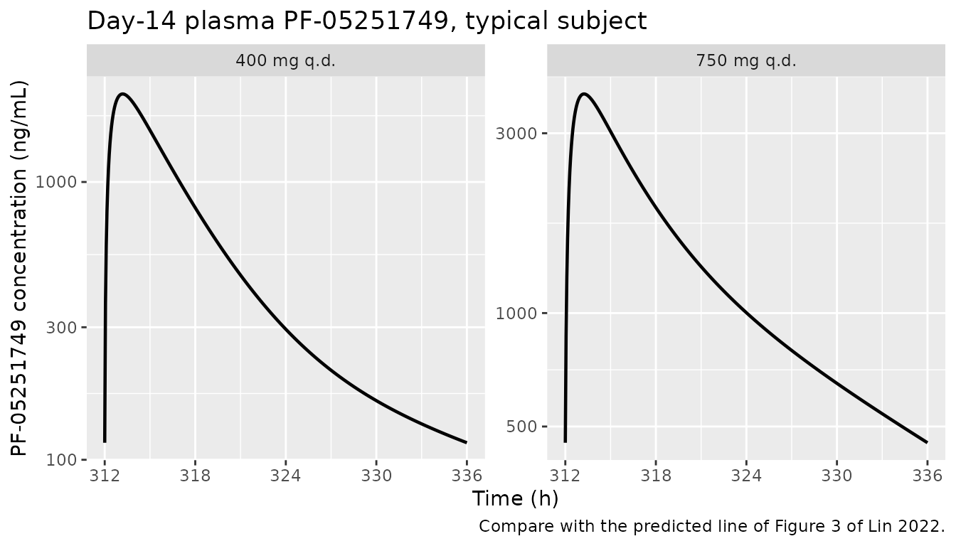
# Replicates the predicted line of Figure 3 of Lin 2022 (day-14 profile of
# PF-05251749 at 400 and 750 mg q.d.). The paper's line is the arithmetic
# mean of a Simcyp virtual population and its 5th/95th percentile band comes
# from unpublished population files, so only the typical profile is shown.
sim |>
  dplyr::filter(time >= 312, time <= 336) |>
  ggplot(aes(time, Cc)) +
  geom_line(linewidth = 0.8) +
  facet_wrap(~treatment, scales = "free_y") +
  scale_y_log10() +
  scale_x_continuous(breaks = seq(312, 336, by = 6)) +
  labs(
    x = "Time (h)", y = "PF-05251749 concentration (ng/mL)",
    title = "Day-14 plasma PF-05251749, typical subject",
    caption = "Compare with the predicted line of Figure 3 of Lin 2022."
  )
sim |>
  dplyr::filter(time <= 384) |>
  ggplot(aes(time, Cc, colour = treatment)) +
  geom_line(linewidth = 0.6) +
  scale_y_log10() +
  scale_x_continuous(breaks = seq(0, 384, by = 48)) +
  labs(
    x = "Time (h)", y = "PF-05251749 concentration (ng/mL)",
    colour = NULL,
    title = "14 days of once-daily dosing and washout"
  )
#> Warning in scale_y_log10(): log-10 transformation introduced infinite values.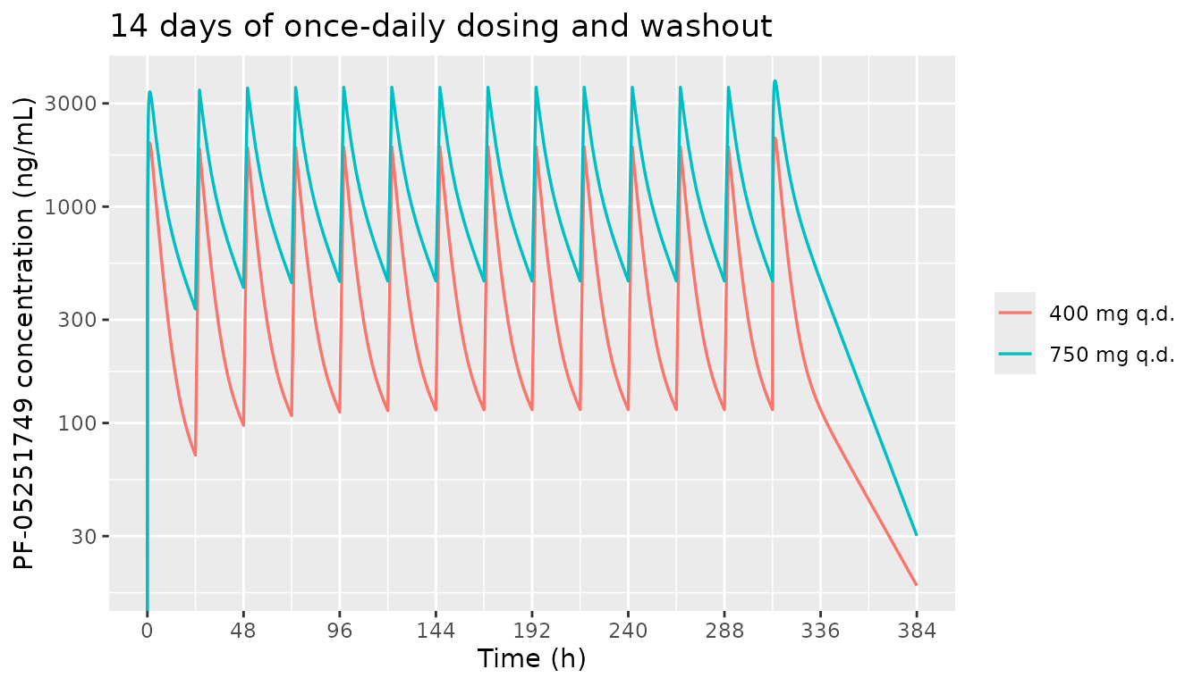
PKNCA validation
conc <- sim |>
  dplyr::filter(!is.na(Cc)) |>
  dplyr::select(id, time, Cc, treatment)

dose <- dplyr::bind_rows(events) |>
  dplyr::filter(evid == 1L) |>
  dplyr::mutate(id = ifelse(treatment == "400 mg q.d.", 1L, 2L)) |>
  dplyr::select(id, time, amt, treatment)

conc_obj <- PKNCA::PKNCAconc(conc, Cc ~ time | treatment + id,
  concu = "ng/mL", timeu = "h"
)
dose_obj <- PKNCA::PKNCAdose(dose, amt ~ time | treatment + id, doseu = "mg")

# Day 1, day 14, and the 48 h after the last dose for the terminal
# half-life (B8001002 sampled to 48 h after the day-14 dose, Figure S2).
intervals <- data.frame(
  start = c(0, 312, 312),
  end = c(24, 336, 360),
  cmax = c(TRUE, TRUE, FALSE),
  tmax = c(TRUE, TRUE, FALSE),
  auclast = c(TRUE, TRUE, FALSE),
  cmin = c(FALSE, TRUE, FALSE),
  half.life = c(FALSE, FALSE, TRUE)
)

nca <- PKNCA::pk.nca(PKNCA::PKNCAdata(conc_obj, dose_obj, intervals = intervals))
nca_df <- as.data.frame(nca)

nca_df |>
  dplyr::filter(
    end - start == 24,
    PPTESTCD %in% c("cmax", "tmax", "auclast", "cmin")
  ) |>
  dplyr::mutate(PPORRES = signif(PPORRES, 4)) |>
  dplyr::select(treatment, start, end, PPTESTCD, PPORRES) |>
  tidyr::pivot_wider(names_from = PPTESTCD, values_from = PPORRES) |>
  dplyr::rename(
    Treatment = treatment, Start = start, End = end,
    "Cmax (ng/mL)" = cmax, "Tmax (h)" = tmax,
    "AUC0-24 (ng*h/mL)" = auclast, "Cmin (ng/mL)" = cmin
  ) |>
knitr::kable(caption = "PKNCA results for day 1 (0-24 h) and day 14 (312-336 h).")| Treatment | Start | End | AUC0-24 (ng*h/mL) | Cmax (ng/mL) | Tmax (h) | Cmin (ng/mL) |
|---|---|---|---|---|---|---|
| 400 mg q.d. | 0 | 24 | 11900 | 1966 | 1.20 | NA |
| 400 mg q.d. | 312 | 336 | 13650 | 2074 | 1.20 | 115.2 |
| 750 mg q.d. | 0 | 24 | 27410 | 3393 | 1.25 | NA |
| 750 mg q.d. | 312 | 336 | 33330 | 3814 | 1.25 | 452.8 |
Comparison against the published predictions
Lin 2022 Table 3 reports the day-14 Simcyp-predicted geometric-mean Cmax and AUCtau and the median Tmax. These are the validation target: the reduction is meant to reproduce the paper’s model, not the clinical data.
published <- tibble::tribble(
  ~treatment, ~start, ~end, ~cmax, ~tmax, ~auclast,
  "400 mg q.d.", 312, 336, 2351, 1.17, 14672,
  "750 mg q.d.", 312, 336, 4094, 1.28, 35833
)

sim_day14 <- nca_df |>
  dplyr::filter(start == 312, end == 336, PPTESTCD %in% c("cmax", "tmax", "auclast"))

cmp <- nlmixr2lib::ncaComparisonTable(
  simulated = sim_day14,
  reference = dplyr::select(published, -start, -end),
  by = "treatment",
  units = c(cmax = "ng/mL", tmax = "h", auclast = "ng*h/mL"),
  tolerance_pct = 20
)

knitr::kable(
  cmp,
  caption = paste(
    "Day-14 typical-subject reduction vs. Lin 2022 Table 3 Simcyp predictions.",
    "* differs from the reference by >20%."
  )
)| NCA parameter | treatment | Reference | Simulated | % diff |
|---|---|---|---|---|
| Cmax (ng/mL) | 400 mg q.d. | 2350 | 2070 | -11.8% |
| Cmax (ng/mL) | 750 mg q.d. | 4090 | 3810 | -6.8% |
| Tmax (h) | 400 mg q.d. | 1.17 | 1.2 | +2.6% |
| Tmax (h) | 750 mg q.d. | 1.28 | 1.25 | -2.3% |
| AUClast (ng*h/mL) | 400 mg q.d. | 14700 | 13700 | -7.0% |
| AUClast (ng*h/mL) | 750 mg q.d. | 35800 | 33300 | -7.0% |
sim_wide <- sim_day14 |>
  dplyr::select(treatment, PPTESTCD, PPORRES) |>
  tidyr::pivot_wider(names_from = PPTESTCD, values_from = PPORRES) |>
  dplyr::inner_join(published, by = "treatment", suffix = c("_sim", "_pub"))

ratios <- sim_wide |>
  dplyr::transmute(
    treatment,
    cmax = cmax_sim / cmax_pub,
    tmax = tmax_sim / tmax_pub,
    auc = auclast_sim / auclast_pub,
    shape = (cmax_sim / auclast_sim) / (cmax_pub / auclast_pub)
  )
knitr::kable(ratios, digits = 3, caption = "Simulated / published ratios.")| treatment | cmax | tmax | auc | shape |
|---|---|---|---|---|
| 400 mg q.d. | 0.882 | 1.026 | 0.93 | 0.948 |
| 750 mg q.d. | 0.932 | 0.977 | 0.93 | 1.002 |
# The models are deterministic, so these bounds are not subject to
# cohort-to-cohort sampling noise.
stopifnot(
  all(abs(ratios$auc - 1) < 0.10),
  all(abs(ratios$tmax - 1) < 0.10),
  all(abs(ratios$cmax - 1) < 0.15),
  all(abs(ratios$shape - 1) < 0.06)
)
Tmax agrees to within 3% at both doses, and AUCtau is 7% below the paper’s prediction at both doses. Cmax is 7% low at 750 mg and 12% low at 400 mg.
The AUCtau offset is the same 7% at both doses, which suggests a population effect rather than a structural one. The reduction’s AUCtau is exactly dose / CLpo by construction (13,652 and 33,333 ngh/mL). The paper’s predicted geometric means sit 7.5% above those values, and they also sit above the observed* geometric means (13,640 and 33,290 ng*h/mL, Table S5) that CLpo was taken from. So the Simcyp virtual population’s geometric-mean oral clearance came out about 7% lower than the CLpo that was entered. A typical-value model cannot carry that. Once the exposure offset is removed, the Cmax/AUCtau ratio, which depends on shape alone, agrees to within 6% at 400 mg and within 0.2% at 750 mg. The remaining 400 mg Cmax gap is mostly the assumed 70 kg reference weight (see the sensitivity analysis below). No parameter was tuned to close it.
Comparison against the observed clinical data
The paper reports the observed steady-state NCA of B8001002 in Table S5. Because CLpo is the observed CL/F, observed AUCtau is matched by construction. The accumulation ratios and the terminal half-life are independent checks of the fitted Vsac and Q.
rac <- nca_df |>
  dplyr::filter(end - start == 24, PPTESTCD %in% c("cmax", "auclast")) |>
  dplyr::select(treatment, start, PPTESTCD, PPORRES) |>
  tidyr::pivot_wider(names_from = c(PPTESTCD, start), values_from = PPORRES) |>
  dplyr::transmute(
    treatment,
    rac_cmax_sim = cmax_312 / cmax_0,
    rac_auc_sim = auclast_312 / auclast_0
  )

thalf <- nca_df |>
  dplyr::filter(PPTESTCD == "half.life") |>
  dplyr::select(treatment, thalf_sim = PPORRES)

observed <- tibble::tribble(
  ~treatment, ~cmax_obs, ~auc_obs, ~rac_cmax_obs, ~rac_auc_obs, ~thalf_obs,
  "400 mg q.d.", 2613, 13640, 1.0, 1.0, 9.9,
  "750 mg q.d.", 4726, 33290, 1.3, 1.2, 11.2
)

sim_wide |>
  dplyr::select(treatment, cmax_sim, auclast_sim) |>
  dplyr::left_join(rac, by = "treatment") |>
  dplyr::left_join(thalf, by = "treatment") |>
  dplyr::left_join(observed, by = "treatment") |>
  dplyr::transmute(
    Treatment = treatment,
    "Cmax sim" = round(cmax_sim), "Cmax obs" = cmax_obs,
    "AUCtau sim" = round(auclast_sim), "AUCtau obs" = auc_obs,
    "Rac,Cmax sim" = round(rac_cmax_sim, 2), "Rac,Cmax obs" = rac_cmax_obs,
    "Rac,AUC sim" = round(rac_auc_sim, 2), "Rac,AUC obs" = rac_auc_obs,
    "t1/2 sim (h)" = round(thalf_sim, 1), "t1/2 obs (h)" = thalf_obs
  ) |>
  knitr::kable(caption = paste(
    "Typical-subject reduction vs. B8001002 observed day-14 geometric means",
    "(Table S5; Rac geometric mean, t1/2 arithmetic mean)."
))| Treatment | Cmax sim | Cmax obs | AUCtau sim | AUCtau obs | Rac,Cmax sim | Rac,Cmax obs | Rac,AUC sim | Rac,AUC obs | t1/2 sim (h) | t1/2 obs (h) |
|---|---|---|---|---|---|---|---|---|---|---|
| 400 mg q.d. | 2074 | 2613 | 13651 | 13640 | 1.06 | 1.0 | 1.15 | 1.0 | 17.9 | 9.9 |
| 750 mg q.d. | 3814 | 4726 | 33331 | 33290 | 1.12 | 1.3 | 1.22 | 1.2 | 12.1 | 11.2 |
At 750 mg the AUC accumulation ratio and the terminal half-life agree with the observed values (1.22 against 1.2, and 12.1 h against 11.2 h), while the Cmax accumulation ratio is lower (1.12 against 1.3). At 400 mg the reduction accumulates slightly more than observed (Rac,AUC 1.15 against 1.0), and its terminal half-life over 0-48 h after the last dose is longer than the observed 9.9 h, because the slower SAC exchange of the 400 mg model (Q 5.8 L/h, against 11 L/h at 750 mg) leaves a shallow late phase. The paper’s own predicted 400 mg line in Figure 3 shows the same shallow decline: it falls by less than half between 12 and 24 h after the dose, while the observed means fall by more. So this is inherited from the fitted Vsac and Q, not introduced by the reduction. The observed Cmax is higher than both the reduction and the paper’s own prediction (Table 3 predicted/observed 0.90 and 0.87), and that gap also comes from the source model.
Sensitivity to the two unprinted constants
Hepatic blood flow and the reference body weight are not printed in Lin 2022. The table below varies each one around the values used here and reports the day-14 Cmax relative to Table 3.
reduce_cmax <- function(dose, clpo, vsac, q, bw, qh_val) {
  fh <- qh_val / (qh_val + clpo / bp)
  m <- readModelDb(ifelse(dose == 400, "Lin_2022_PF05251749_400mg",
    "Lin_2022_PF05251749_750mg"
  ))
  m <- rxode2::ini(rxode2::rxode(m),
    lcl = log(fh * clpo), lfdepot = log(fh),
    lvc = log((vss_per_kg - vsac) * bw - liver_l), lvp = log(vsac * bw)
  )
  ev <- make_subject(1L, dose, "x") |> dplyr::filter(evid == 1L | time >= 312)
  s <- as.data.frame(rxode2::rxSolve(m, events = ev))
  max(s$Cc[s$time >= 312 & s$time <= 336])
}

sens <- tidyr::expand_grid(bw = c(65, 70, 75), qh_val = c(80, 90, 100)) |>
  dplyr::rowwise() |>
  dplyr::mutate(
    "Cmax 400 / Table 3" = reduce_cmax(400, 29.3, 1.6, 5.8, bw, qh_val) / 2351,
    "Cmax 750 / Table 3" = reduce_cmax(750, 22.5, 1.3, 11, bw, qh_val) / 4094
  ) |>
  dplyr::ungroup() |>
  dplyr::rename("Body weight (kg)" = bw, "QH (L/h)" = qh_val)
#> ℹ change initial estimate of `lcl` to `2.95676475226054`
#> ℹ change initial estimate of `lfdepot` to `-0.420822763762484`
#> ℹ change initial estimate of `lvc` to `4.56280533521032`
#> ℹ change initial estimate of `lvp` to `4.64439089914137`
#> ℹ change initial estimate of `lcl` to `2.99567810090575`
#> ℹ change initial estimate of `lfdepot` to `-0.381909415117274`
#> ℹ change initial estimate of `lvc` to `4.56280533521032`
#> ℹ change initial estimate of `lvp` to `4.64439089914137`
#> ℹ change initial estimate of `lcl` to `3.02793718702125`
#> ℹ change initial estimate of `lfdepot` to `-0.349650329001768`
#> ℹ change initial estimate of `lvc` to `4.56280533521032`
#> ℹ change initial estimate of `lvp` to `4.64439089914137`
#> ℹ change initial estimate of `lcl` to `2.95676475226054`
#> ℹ change initial estimate of `lfdepot` to `-0.420822763762484`
#> ℹ change initial estimate of `lvc` to `4.638140637658`
#> ℹ change initial estimate of `lvp` to `4.71849887129509`
#> ℹ change initial estimate of `lcl` to `2.99567810090575`
#> ℹ change initial estimate of `lfdepot` to `-0.381909415117274`
#> ℹ change initial estimate of `lvc` to `4.638140637658`
#> ℹ change initial estimate of `lvp` to `4.71849887129509`
#> ℹ change initial estimate of `lcl` to `3.02793718702125`
#> ℹ change initial estimate of `lfdepot` to `-0.349650329001768`
#> ℹ change initial estimate of `lvc` to `4.638140637658`
#> ℹ change initial estimate of `lvp` to `4.71849887129509`
#> ℹ change initial estimate of `lcl` to `2.95676475226054`
#> ℹ change initial estimate of `lfdepot` to `-0.420822763762484`
#> ℹ change initial estimate of `lvc` to `4.7081959782992`
#> ℹ change initial estimate of `lvp` to `4.78749174278205`
#> ℹ change initial estimate of `lcl` to `2.99567810090575`
#> ℹ change initial estimate of `lfdepot` to `-0.381909415117274`
#> ℹ change initial estimate of `lvc` to `4.7081959782992`
#> ℹ change initial estimate of `lvp` to `4.78749174278205`
#> ℹ change initial estimate of `lcl` to `3.02793718702125`
#> ℹ change initial estimate of `lfdepot` to `-0.349650329001768`
#> ℹ change initial estimate of `lvc` to `4.7081959782992`
#> ℹ change initial estimate of `lvp` to `4.78749174278205`
#> ℹ change initial estimate of `lcl` to `2.77576837515716`
#> ℹ change initial estimate of `lfdepot` to `-0.337746934053213`
#> ℹ change initial estimate of `lvc` to `4.74798832300435`
#> ℹ change initial estimate of `lvp` to `4.43675153436313`
#> ℹ change initial estimate of `lcl` to `2.80813365965919`
#> ℹ change initial estimate of `lfdepot` to `-0.305381649551182`
#> ℹ change initial estimate of `lvc` to `4.74798832300435`
#> ℹ change initial estimate of `lvp` to `4.43675153436313`
#> ℹ change initial estimate of `lcl` to `2.83480190674135`
#> ℹ change initial estimate of `lfdepot` to `-0.27871340246902`
#> ℹ change initial estimate of `lvc` to `4.74798832300435`
#> ℹ change initial estimate of `lvp` to `4.43675153436313`
#> ℹ change initial estimate of `lcl` to `2.77576837515716`
#> ℹ change initial estimate of `lfdepot` to `-0.337746934053213`
#> ℹ change initial estimate of `lvc` to `4.82311625375497`
#> ℹ change initial estimate of `lvp` to `4.51085950651685`
#> ℹ change initial estimate of `lcl` to `2.80813365965919`
#> ℹ change initial estimate of `lfdepot` to `-0.305381649551182`
#> ℹ change initial estimate of `lvc` to `4.82311625375497`
#> ℹ change initial estimate of `lvp` to `4.51085950651685`
#> ℹ change initial estimate of `lcl` to `2.83480190674135`
#> ℹ change initial estimate of `lfdepot` to `-0.27871340246902`
#> ℹ change initial estimate of `lvc` to `4.82311625375497`
#> ℹ change initial estimate of `lvp` to `4.51085950651685`
#> ℹ change initial estimate of `lcl` to `2.77576837515716`
#> ℹ change initial estimate of `lfdepot` to `-0.337746934053213`
#> ℹ change initial estimate of `lvc` to `4.89299224864079`
#> ℹ change initial estimate of `lvp` to `4.5798523780038`
#> ℹ change initial estimate of `lcl` to `2.80813365965919`
#> ℹ change initial estimate of `lfdepot` to `-0.305381649551182`
#> ℹ change initial estimate of `lvc` to `4.89299224864079`
#> ℹ change initial estimate of `lvp` to `4.5798523780038`
#> ℹ change initial estimate of `lcl` to `2.83480190674135`
#> ℹ change initial estimate of `lfdepot` to `-0.27871340246902`
#> ℹ change initial estimate of `lvc` to `4.89299224864079`
#> ℹ change initial estimate of `lvp` to `4.5798523780038`
knitr::kable(sens, digits = 3, caption = "Day-14 Cmax ratio vs. reference weight and hepatic blood flow.")| Body weight (kg) | QH (L/h) | Cmax 400 / Table 3 | Cmax 750 / Table 3 |
|---|---|---|---|
| 65 | 80 | 0.905 | 0.956 |
| 65 | 90 | 0.932 | 0.977 |
| 65 | 100 | 0.955 | 0.996 |
| 70 | 80 | 0.857 | 0.912 |
| 70 | 90 | 0.882 | 0.932 |
| 70 | 100 | 0.904 | 0.949 |
| 75 | 80 | 0.815 | 0.873 |
| 75 | 90 | 0.839 | 0.891 |
| 75 | 100 | 0.859 | 0.907 |
Hepatic blood flow matters little: a 10 L/h change in QH moves Cmax by about 3%, and it cannot change AUCtau, because QH changes F and the systemic clearance together. Body weight matters more, because the volumes are given per kg. The 70 kg reference is a convention, not a fitted value, and it was not chosen to match Table 3.
The induction layer and the midazolam interaction
The induction model used the linear-fit in vitro CYP3A mRNA induction slope (Equation 2 of Lin 2022, fold induction = 1 + slope x C). Slopes were estimated in three hepatocyte donor lots (Table S2: 0.124, 0.385 and 0.036 per uM). Each was calibrated against rifampin, by multiplying it by the ratio of rifampin’s in vivo slope (21.9 per uM) to its in vitro slope in the same lot. The most potent calibrated slope, 0.18 per uM from lot HC7-4 (Table S1), was used in Simcyp. With it, Table 4 predicts midazolam Cmax and AUCinf geometric-mean ratios of 0.86 and 0.83 at 400 mg q.d., and 0.71 and 0.66 at 750 mg q.d.
tibble::tibble(
  Lot = c("HH1025", "HC7-4", "FOS"),
  in_vitro = c(0.124, 0.385, 0.0361),
  rif_in_vitro = c(24.45, 46.5, 52.3),
  printed = c(0.11, 0.18, 0.015)
) |>
  dplyr::mutate(recomputed = in_vitro * 21.9 / rif_in_vitro) |>
  dplyr::rename(
    "PF-05251749 in vitro slope (/uM)" = in_vitro,
    "Rifampin in vitro slope (/uM)" = rif_in_vitro,
    "Calibrated slope, Table S1 (/uM)" = printed,
    "Calibrated slope, recomputed (/uM)" = recomputed
  ) |>
knitr::kable(digits = 3, caption = "Rifampin calibration of the induction slopes (Table S1).")| Lot | PF-05251749 in vitro slope (/uM) | Rifampin in vitro slope (/uM) | Calibrated slope, Table S1 (/uM) | Calibrated slope, recomputed (/uM) |
|---|---|---|---|---|
| HH1025 | 0.124 | 24.45 | 0.110 | 0.111 |
| HC7-4 | 0.385 | 46.50 | 0.180 | 0.181 |
| FOS | 0.036 | 52.30 | 0.015 | 0.015 |
This layer is not encoded. In Simcyp the calibrated slope drives a CYP3A enzyme-turnover equation through the unbound concentration in the liver and the gut wall. The enzyme degradation rate constants that set its time course, and the gut-wall concentration, are Simcyp defaults that Lin 2022 does not print. The victim drug, midazolam, is a Simcyp library compound with no parameter given in the paper. Neither the enzyme time course nor the midazolam exposure can therefore be rebuilt from the paper. The 4-beta-hydroxycholesterol/cholesterol ratios in Table 1 are least-squares-mean fold changes from a statistical comparison, not a model, and the authors did not undertake an exposure-response analysis of them.
Assumptions and deviations
- The Simcyp platform model is not encoded. Each file is a two-compartment reduction of the minimal PBPK model with an SAC. The liver and portal vein are lumped into the systemic compartment, and hepatic first-pass extraction is folded into the bioavailability through the well-stirred model. The reductions are validated by reproducing the paper’s predictions, not its internal structure.
- Hepatic blood flow (90 L/h) and liver volume (1.648 L) are not printed in Lin 2022. Both are the standard Simcyp healthy-adult values printed in Hanley 2024 Appendix S1. A 10 L/h change in QH moves Cmax by about 3% (see the sensitivity table), and the liver volume changes the systemic volume by about 1.5%.
- fG = 1. Table 2 gives F u,gut = 1 and an in vivo clearance with no enzyme pathways, so no gut-wall extraction is applied. fa = 1 is the authors’ assumption (Table 2).
-
The V_sys convention is imported, not sourced. The
systemic volume is taken as (Vss - Vsac) x body weight - liver volume,
the convention used for other Simcyp minimal-PBPK reductions in this
package (
Hanley_2024_brigatinib). The reduction’s own steady-state volume is close to, but not identical to, the Table 2 Vss. - A 70 kg reference weight is used for the L/kg volumes. The paper does not state the weight of its virtual population. The B8001002 mean weight was 76.4 kg (Table S3), which would lower Cmax by about 6%.
- Two files, as the authors built two models. The 400 and 750 mg base models share Vss and ka but have separate CLpo, Vsac and Q (Table 2), because PF-05251749 PK was less than dose-proportional above 200 mg q.d. Neither model should be used to interpolate to other doses. The Simcyp models were qualified at steady state only.
-
No inter-individual variability and no residual
error. The %CV values in Table 3 are the spread of the Simcyp
virtual population. There are no etas, and
propSdis zero. - The predicted geometric means sit 7% above dose / CLpo. The paper’s virtual population had a geometric-mean clearance about 7% below the entered CLpo. The typical-value reduction uses CLpo itself.
-
Table 2 permeability. Table 2 labels the
permeability input as MDCK P app 30.4 x 10^-6 cm/s, while the Methods
text gives the RRCK permeability as 31.6 x 10^-6 cm/s. Absorption here
is driven by the first-order
kaalone, so the discrepancy does not affect either model. - The CYP3A induction and midazolam DDI layer are not encoded, for the reasons given above.