Dolutegravir maternal-fetal pregnancy PBPK (Freriksen 2020)
Source:vignettes/articles/Freriksen_2020_dolutegravir_pregnancy_pbpk.Rmd
Freriksen_2020_dolutegravir_pregnancy_pbpk.RmdModel and source
Freriksen et al. (2020, Clin Pharmacol Ther 107:1352-1361, doi:10.1002/cpt.1748) built a pregnancy physiologically based pharmacokinetic (p-PBPK) model for the HIV integrase inhibitor dolutegravir in Berkeley Madonna, and extended it with a fetoplacental unit whose placental transfer clearances were measured in ex vivo dual-side human cotyledon perfusions. The model simulates maternal plasma, fetal plasma and amniotic-fluid concentrations after 50 mg once daily at 34 weeks of gestation.
The authors deposited the complete Berkeley Madonna script as Supplementary File S2, together with the compound table (Table S1) and the gestational-age regressions (Table S2). This model file is a line-by-line port of that script.
- Maternal body: 15 perfusion-rate-limited states (oral depot = gut lumen, gut wall, lung, adipose, bone, brain, heart, kidney, muscle, skin, spleen, liver, rest of body, arterial and venous blood). Kp values were predicted by Rodgers-Rowland in Simcyp v17 and are printed in Table S1.
- Liver: well-stirred, with UGT1A1 + CYP3A4 intrinsic clearance scaled up from recombinant-enzyme data and multiplied by an empirical scaling factor SF = 65. The authors fitted SF against the Min 2010 healthy-volunteer single-ascending-dose data.
- Placenta: a barrier, not a compartment. The apparent cotyledon clearance (1.03 mL/min in each direction) is converted to an unbound clearance with the perfusion-buffer fraction unbound, then scaled back to in vivo using the blood fraction unbound on each side and 30 cotyledons per placenta.
- Fetus: fetal blood, rest of fetal body, and amniotic fluid. Amniotic-fluid exchange uses literature fluid flows scaled by a factor A_SF = 3.
mod <- readModelDb("Freriksen_2020_dolutegravir_pregnancy_pbpk")
mod_ui <- rxode2::rxode2(mod)
Population
The model describes one typical pregnant woman at 34 weeks of gestation, not a population. The authors matched covariates to the mean values of the clinical studies (Methods, “Physiologically-based pharmacokinetic modeling”). Her Table S2 regressions give a body weight of 73.7 kg and a cardiac output of 400.4 L/h at 34 weeks. The simulations were compared with:
- mean third-trimester maternal profiles from the PANNA network (n = 15) and IMPAACT P1026s (n = 28);
- cord-to-maternal plasma ratios from PANNA (n = 10), Rimawi et al. (n = 3) and IMPAACT (n = 23);
- one published amniotic-fluid concentration (0.03 ug/mL).
The paper has no between-subject variability and no residual-error model, so the model file has none either.
Source trace
| Element | Value | Source |
|---|---|---|
| ODE system (all 18 states) | – | Supplementary File S2, ‘DIFFERENTIAL EQUATIONS’; Methods equations; Figure 1 |
ka, Fabs
|
2.25 1/h, 0.804 | Table S1 ‘Absorption’; File S2 |
| 12 maternal Kp + fetal rest-of-body Kp | 0.0730-0.3195 | Table S1 ‘Distribution’; File S2 |
fu (pregnant), fu_fet
|
0.0049, 0.0036 | Table S1 ‘Fraction unbound in plasma’ |
bpr, bpr_fet
|
0.535, 0.441 | Table S1 ‘Blood:plasma ratio’ |
CLint UGT1A1, CYP3A4 |
2.7, 0.56 uL/min/mg | Table S1 ‘Metabolism/elimination’ |
fumic, MPPGL
|
0.817, 39.79067 mg/g | Table S1; File S2 |
| Liver scaling factor SF | 65 | Table S1; Methods (‘refined well-stirred model’) |
| CYP3A4 / UGT1A1 induction | 100 + 2.9826 GA - 0.0741 GA^2 (%) | Table S2; File S2 (UGT1A1 assumed equal to CYP3A4) |
| Cotyledon clearances, buffer fu, Ncot | 1.03 / 1.03 mL/min, 0.048 / 0.043, 30 | Table 1; File S2 |
| Placental scaling equation | CL_plac = CL_app / fu_perf * fu_b * Ncot | Methods equations; File S2 |
| Maternal BW, CO | 61.1 + 0.24098 GA + 0.0038 GA^2; 301 + 5.916 GA - 0.088 GA^2 | Table S2; File S2 |
| Fractional volumes and flows | per organ | File S2 (‘Gaohua 2012’, ‘Simcyp v17 healthy female’) |
| Fetal volume, fetal blood, amniotic volume | Gompertz, linear, quintic in GA | Table S2; File S2 |
| Fetal cardiac output, fraction to placenta | 553 * VtotalF * 0.06; exp(…) / 100 | Table S2; File S2 |
| Amniotic exchange flows and A_SF | 0.275 / 0.774 / 0.350 L/day; A_SF = 3 | File S2 (Underwood 2005) |
| Validation targets | maternal C0 0.99, fetal Ctrough 1.50 ug/mL, C:M 0.57-1.51, amniotic 0.025-0.039 ug/mL | Results, ‘PBPK model in pregnant subjects’ |
Simulation: 50 mg once daily at 34 weeks (Figure 4)
The deposited script gives seven 50 mg doses at 24 h intervals and
simulates to 168 h. The same regimen is used here. Observation rows are
placed on the venous-blood state, and rxode2 returns the algebraic
outputs Cc (maternal venous plasma),
Cplasma_fet and Camniotic at each row.
ev <- rxode2::et(amt = 50, cmt = "depot", ii = 24, addl = 6) |>
  rxode2::et(seq(0, 168, by = 0.05), cmt = "venous") |>
  as.data.frame()
ev$GA <- 34
sim <- as.data.frame(rxode2::rxSolve(mod_ui, ev, returnType = "data.frame"))
sim |>
  select(time, `Maternal plasma` = Cc, `Fetal plasma` = Cplasma_fet, `Amniotic fluid` = Camniotic) |>
  pivot_longer(-time, names_to = "matrix", values_to = "conc") |>
  ggplot(aes(time, conc, linetype = matrix, colour = matrix)) +
  geom_line() +
  scale_colour_manual(values = c("Maternal plasma" = "black", "Fetal plasma" = "grey55", "Amniotic fluid" = "black")) +
  scale_linetype_manual(values = c("Maternal plasma" = "solid", "Fetal plasma" = "solid", "Amniotic fluid" = "dotted")) +
  labs(x = "Time (h)", y = "Dolutegravir (ug/mL)", colour = NULL, linetype = NULL) +
  theme_bw()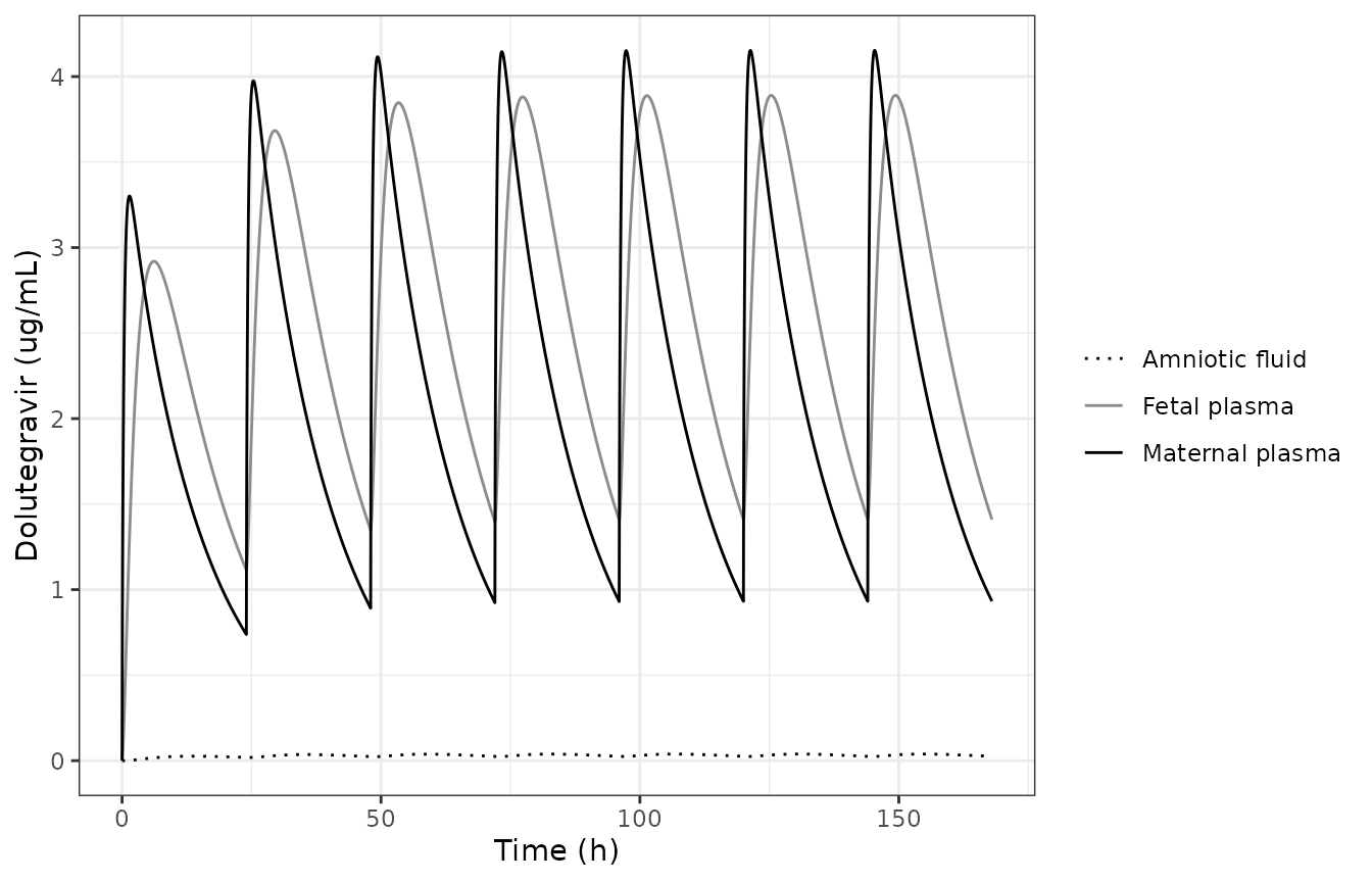
Replicates Figure 4 of Freriksen 2020: maternal plasma, fetal plasma and amniotic-fluid dolutegravir after 50 mg once daily at 34 weeks of gestation.
Comparison with the published numbers
The Results text gives the following deterministic values for the last dosing interval (144-168 h). All of them come from the same single-subject solve.
ss <- sim |> filter(time >= 144) |> mutate(tad = time - 144, ratio = Cplasma_fet / Cc)
trough <- ss |> filter(abs(tad - 24) < 1e-6)
hourly <- ss |> filter(abs(tad - round(tad)) < 1e-6)

checks <- data.frame(
  Quantity = c(
    "Maternal plasma C0 (ug/mL)",
    "Fetal plasma Ctrough (ug/mL)",
    "Fetal:maternal plasma ratio, max over interval",
    "Fetal:maternal plasma ratio, min over interval (1 h grid)",
    "Amniotic fluid, min over interval (ug/mL)",
    "Amniotic fluid, max over interval (ug/mL)"
  ),
  Published = c(0.99, 1.50, 1.51, 0.57, 0.025, 0.039),
  Simulated = c(
    trough$Cc, trough$Cplasma_fet, max(ss$ratio), min(hourly$ratio),
    min(ss$Camniotic), max(ss$Camniotic)
  )
) |>
  mutate(`% diff` = round(100 * (Simulated / Published - 1), 1), Simulated = signif(Simulated, 3))
knitr::kable(checks)| Quantity | Published | Simulated | % diff |
|---|---|---|---|
| Maternal plasma C0 (ug/mL) | 0.990 | 0.9320 | -5.8 |
| Fetal plasma Ctrough (ug/mL) | 1.500 | 1.4100 | -6.0 |
| Fetal:maternal plasma ratio, max over interval | 1.510 | 1.5100 | 0.1 |
| Fetal:maternal plasma ratio, min over interval (1 h grid) | 0.570 | 0.5380 | -5.6 |
| Amniotic fluid, min over interval (ug/mL) | 0.025 | 0.0245 | -2.0 |
| Amniotic fluid, max over interval (ug/mL) | 0.039 | 0.0386 | -1.0 |
stopifnot(
  # Maternal and fetal troughs: a mis-transcribed SF, fu, Kp or placental
  # clearance moves these by tens of percent (SF 65 -> 60 alone gives +17%).
  abs(trough$Cc / 0.99 - 1) < 0.10,
  abs(trough$Cplasma_fet / 1.50 - 1) < 0.10,
  # The fetal:maternal ratio depends only on the placental layer.
  abs(max(ss$ratio) / 1.51 - 1) < 0.02,
  # Amniotic-fluid range.
  abs(min(ss$Camniotic) - 0.025) < 0.002,
  abs(max(ss$Camniotic) - 0.039) < 0.002
)
The simulated maternal and fetal troughs at 24 h after the last dose are 6% below the published 0.99 and 1.50 ug/mL. One hour earlier (23 h after the dose) the model gives 0.995 and 1.5 ug/mL. Both round to the published values, and the ratio between them (1.51) matches the paper. The uniform 6% offset in both matrices therefore points to the maternal disposition layer, or to when the published trough was read off the output, and not to the placental transfer. The trough is very sensitive to SF: changing it from 65 to 60 raises the trough by 17%. A 6% offset is within the rounding of the printed inputs, so no parameter was adjusted.
The smallest fetal:maternal ratio (just after the maternal peak) is
0.54 on the script’s 1 h output grid (DTOUT = 1), against a
published 0.57. The fetal peak lags the maternal peak, so this minimum
depends on how finely the output is sampled.
Mass balance
At steady state, the drug eliminated by the liver over one dosing
interval must equal the bioavailable dose, 50 mg x 0.804 = 40.2 mg. The
paper has no other elimination route. The same solve gives the integrand
cl_liver * cu_liver. Integrating it over the last interval
checks the ODE topology directly (every flow in must have a matching
flow out).
PKNCA: steady-state interval (day 7)
NCA is run on the last dosing interval, with time re-anchored to the start of the interval. Two separate NCA blocks are used, one for maternal plasma and one for fetal plasma.
nca_conc <- ss |>
  select(tad, Cc, Cplasma_fet) |>
  pivot_longer(c(Cc, Cplasma_fet), names_to = "matrix", values_to = "conc") |>
  mutate(id = 1L, treatment = "50 mg QD, GA 34 wk") |>
  filter(!is.na(conc))
nca_dose <- data.frame(id = 1L, treatment = "50 mg QD, GA 34 wk", tad = 0, amt = 50)
intervals <- data.frame(start = 0, end = 24, cmax = TRUE, tmax = TRUE, cmin = TRUE, auclast = TRUE, cav = TRUE)

run_nca <- function(m) {
  o_conc <- PKNCA::PKNCAconc(filter(nca_conc, matrix == m), conc ~ tad | treatment + id)
  o_dose <- PKNCA::PKNCAdose(nca_dose, amt ~ tad | treatment + id)
  res <- PKNCA::pk.nca(PKNCA::PKNCAdata(o_conc, o_dose, intervals = intervals))
  as.data.frame(res$result) |> mutate(matrix = m)
}
nca_res <- bind_rows(run_nca("Cc"), run_nca("Cplasma_fet"))
nca_res |>
  select(matrix, PPTESTCD, PPORRES) |>
  pivot_wider(names_from = PPTESTCD, values_from = PPORRES) |>
  mutate(across(where(is.numeric), ~ signif(.x, 3))) |>
  rename(
    "Matrix" = matrix, "Cmax (ug/mL)" = cmax, "Tmax (h)" = tmax, "Cmin (ug/mL)" = cmin,
    "AUC0-24 (ug*h/mL)" = auclast, "Cav (ug/mL)" = cav
  ) |>
knitr::kable()| Matrix | AUC0-24 (ug*h/mL) | Cmax (ug/mL) | Cmin (ug/mL) | Tmax (h) | Cav (ug/mL) |
|---|---|---|---|---|---|
| Cc | 53.7 | 4.15 | 0.932 | 1.35 | 2.24 |
| Cplasma_fet | 65.4 | 3.89 | 1.410 | 5.35 | 2.73 |
The paper reports only the troughs, so the comparison table is
limited to cmin. That is the trough (C0) for both matrices,
because at steady state the fetal minimum also falls at the time of
dosing.
sim_cmp <- nca_res |>
  filter(PPTESTCD == "cmin") |>
  select(matrix, PPTESTCD, PPORRES)
ref_cmp <- data.frame(matrix = c("Cc", "Cplasma_fet"), cmin = c(0.99, 1.50))
tbl <- nlmixr2lib::ncaComparisonTable(sim_cmp, ref_cmp, by = "matrix", units = c(cmin = "ug/mL"))
knitr::kable(tbl)| NCA parameter | matrix | Reference | Simulated | % diff |
|---|---|---|---|---|
| Cmin (ug/mL) | Cc | 0.99 | 0.932 | -5.9% |
| Cmin (ug/mL) | Cplasma_fet | 1.5 | 1.41 | -6.0% |
Gestational age
Gestational age (GA) drives every physiological
regression of Table S2, so the model accepts it as a covariate. The
paper simulated and validated 34 weeks only. The protein-binding inputs
fu and fu_fet are the 34-week values and do
not change with GA. The table below is therefore an extrapolation that
shows the physiological drift only.
ga_tab <- lapply(c(30, 34, 38), function(g) {
  e <- ev
  e$GA <- g
  s <- as.data.frame(rxode2::rxSolve(mod_ui, e, returnType = "data.frame"))
  s |>
    filter(abs(time - 168) < 1e-6) |>
    transmute(`GA (weeks)` = g, `Maternal C0` = signif(Cc, 3), `Fetal Ctrough` = signif(Cplasma_fet, 3))
}) |> bind_rows()
knitr::kable(ga_tab)| GA (weeks) | Maternal C0 | Fetal Ctrough |
|---|---|---|
| 30 | 0.839 | 1.20 |
| 34 | 0.932 | 1.41 |
| 38 | 1.080 | 1.70 |
Assumptions and deviations
-
Deposited script over prose. Every value and
equation is taken from Supplementary File S2 (Berkeley Madonna script)
and Tables 1, S1 and S2. Berkeley Madonna identifiers are
case-insensitive, so the script’s
Clplac_mfandCLplac_mf(andKa/ka) are the same variable. The script’s en-dash in the liver equation is a minus sign. -
Kp scalar. The script multiplies each maternal Kp
by
KpScalar = 1. The factor is omitted here because it is 1. - Enzyme induction. The script applies the same gestational-age factor to CYP3A4 and UGT1A1 (the paper assumes UGT1A1 induction is proportional to CYP3A4). The model applies it once to the summed intrinsic clearance, which is algebraically identical.
-
Hepatic unbound concentration. As in the script,
the unbound liver concentration is
C_liver * fu(plasma fraction unbound), notC_liver / Kp * fu. -
Output site. Maternal plasma is venous plasma
(
Cvenous / BP, scriptCven_plasmaM). The paper does not say whether Figure 4 shows venous or arterial plasma. At trough the two agree to 3 significant figures. -
Doses. The script’s
pulse(dose*Fabs, 0, 24)impulse into the gut lumen is encoded as 50 mg bolus doses intodepotwithf(depot) = Fabs. - Trough offset. The simulated maternal and fetal troughs are 6% below the published values (see above). No parameter was tuned.
- Healthy-volunteer model (Figure 3) not reproduced. The nonpregnant model used to fit SF has a different fraction unbound (0.0041) and nonpregnant physiology. Its body weight and cardiac output are not given, and the fetal regressions are undefined at GA = 0, so Figure 3 cannot be reproduced from this file.
- Third trimester only. The fetal-blood regression is negative below about 18.7 weeks, so the model is not valid early in pregnancy.
-
Specimen coding. The amniotic-fluid state is coded
as specimen
tissue, following other gestational PBPK models in the package, because the specimen vocabulary has no amniotic-fluid entry. - No variability. The paper is a single typical-subject forward simulation, with no IIV and no residual-error model.