Model and source
- Citation: Zhu L, Wang H, Sun X, Rao W, Qu W, Zhang Y, Sun L. The Population Pharmacokinetic Models of Tacrolimus in Chinese Adult Liver Transplantation Patients. Journal of Pharmaceutics. 2014;2014:713650. doi:10.1155/2014/713650
- Description: Two-compartment population PK model for oral tacrolimus in Chinese adult liver transplant recipients (Zhu 2014), with first-order absorption, a power-form joint DOSE x POD covariate effect on apparent clearance, log-normal IIV on CL/F, V2/F, Q/F, V3/F, and ka, and proportional residual error. Bioavailability was not estimated; the structural disposition parameters are apparent values (CL/F, V/F, Q/F).
- Article: https://doi.org/10.1155/2014/713650
Population
Zhu 2014 developed the model from 435 whole-blood tacrolimus concentrations collected from 47 Chinese adult liver transplant recipients hospitalised at the Tianjin First Central Hospital between 2008 and 2011 (Table 1). The cohort included 27 male and 20 female adults aged 25-78 years (mean 57.47, median 60). Patients received oral tacrolimus capsules (0.5 mg and 1 mg) as part of a triple-immunosuppression regimen with mycophenolate mofetil and corticosteroids; therapy was initiated at 0.1-0.15 mg/kg twice daily and titrated by therapeutic drug monitoring to a whole-blood trough target of 10-15 ng/mL during the first three posttransplant months. Observed daily doses ranged from 1 to 10.5 mg (median 5 mg). Postoperative day at sampling ranged from 2 to 85 (median 14). Body weight was not collected because of extensive missing data among inpatients; eleven other covariates (demographics plus liver-function, renal-function, and haematological indices) were screened, but only DOSE and POD on apparent oral clearance survived stepwise forward inclusion (alpha = 0.01) and backward elimination (alpha = 0.005). Tacrolimus concentrations were measured by microparticle enzyme immunoassay (MEIA, IMx platform; LLOQ 1.5 ng/mL, linear range 1.5-30 ng/mL) which cross-reacts with three tacrolimus metabolites (M-II, M-III, M-V); the assay therefore reports the sum of parent drug plus those three metabolites.
The same information is available programmatically via
readModelDb("Zhu_2014_tacrolimus")$population.
Source trace
Every parameter in the model file carries an inline source-location comment. The table below collects the entries in one place.
| Equation / parameter | Value | Source location |
|---|---|---|
lka (ka) |
0.723 1/h | Table 4, Parameter estimate column, ka row |
lcl (theta_CL/F coefficient at DOSE=1, POD=1) |
11.2 L/h | Table 4, Parameter estimate column, CL/F row |
lvc (V2/F, central) |
406 L | Table 4, Parameter estimate column, V2 row |
lq (Q/F) |
57.3 L/h | Table 4, Parameter estimate column, Q row |
lvp (V3/F, peripheral) |
503 L | Table 4, Parameter estimate column, V3 row |
e_dose_cl (theta_DOSE) |
0.371 | Table 4, Parameter estimate column, theta_DOSE row |
e_pod_cl (theta_POD) |
0.127 | Table 4, Parameter estimate column, theta_POD row |
| IIV CL/F (omega^2 = log(0.162^2 + 1) = 0.02591) | 16.2% CV | Table 4, Parameter estimate column, omega CL/F row |
| IIV V2/F (omega^2 = log(1.63^2 + 1) = 1.29657) | 163% CV | Table 4, Parameter estimate column, omega V2/F row |
| IIV Q/F (omega^2 = log(0.197^2 + 1) = 0.03808) | 19.7% CV | Table 4, Parameter estimate column, omega Q/F row |
| IIV V3/F (omega^2 = log(1.99^2 + 1) = 1.60139) | 199% CV | Table 4, Parameter estimate column, omega V3/F row |
| IIV ka (omega^2 = log(0.743^2 + 1) = 0.43972) | 74.3% CV | Table 4, Parameter estimate column, omega ka row |
| Proportional residual error | 26.54% | Table 4, Parameter estimate column, sigma row |
| Bioavailability F | not estimated | Methods Section 2.4 (“the bioavailability (F) and absorption with a lag time could not be determined”) |
| Covariate equation for CL/F | – | Equation (3) on page 4: CL/F = theta_CL/F * DOSE^theta_DOSE * POD^theta_POD |
| IIV log-normal form | – | Equation (1) on page 3: theta_ij = theta * exp(eta_ij) |
| Proportional residual error | – | Equation (2) on page 3: Y = IPRED * (1 + epsilon) |
| 2-compartment structure with first-order absorption | – | Section 3.2 paragraph 1 |
Virtual cohort
The published dataset is not openly available, so the virtual cohort below mirrors the demographics in Zhu 2014 Table 1. Because Zhu 2014 did not collect body weight and reports neither bioavailability nor absorption-lag time, the simulated cohort carries only the two covariates the model consumes (DOSE and POD) along with a categorical posttransplant-phase label used downstream for stratified summaries.
Three POD strata are simulated to reproduce the paper’s recovery-of-CL discussion: an early phase (POD 5 d), a mid phase (POD 14 d – cohort median), and a late phase (POD 60 d). All cohorts receive the cohort-median daily dose (5 mg) split into 2.5 mg twice daily (the per-protocol oral schedule of Zhu 2014; doses were dispensed as 0.5 mg and 1 mg capsules).
set.seed(20140213)

n_per_pod <- 200L

make_cohort <- function(n, pod_value, label, id_offset = 0L) {
  tibble(
    id    = id_offset + seq_len(n),
    DOSE  = 5,            # cohort-median daily total tacrolimus dose (mg/d)
    POD   = pod_value,    # posttransplant day at the simulated trough
    cohort = label
  )
}

demo <- bind_rows(
  make_cohort(n_per_pod, pod_value =  5, label = "POD  5 d (early)",        id_offset = 0L),
  make_cohort(n_per_pod, pod_value = 14, label = "POD 14 d (median)",       id_offset = 1L * n_per_pod),
  make_cohort(n_per_pod, pod_value = 60, label = "POD 60 d (steady-state)", id_offset = 2L * n_per_pod)
)
stopifnot(!anyDuplicated(demo$id))
Simulation
Each subject receives 2.5 mg oral tacrolimus every 12 hours for 5 simulated days (10 doses). The observation grid covers 0-12 h around the first dose (early absorption profile) and a dense window around the final 12-h interval (steady-state trough sampling).
build_events <- function(demo, dose_mg = 2.5, sim_hours = 120) {
  # Twice-daily dosing for 5 days (10 doses).
  doses <- demo |>
    mutate(amt = dose_mg, evid = 1L, cmt = "depot",
           ii = 12, addl = 9L, time = 0) |>
    select(id, time, amt, evid, cmt, ii, addl, cohort, DOSE, POD)

  # Observations: every 30 min for the first 12 h (early profile) and
  # every 30 min over the last 12-h interval (steady-state profile).
  obs_times <- sort(unique(c(seq(0, 12, by = 0.5),
                             seq(sim_hours - 12, sim_hours, by = 0.5))))
  obs <- demo |>
    select(id, cohort, DOSE, POD) |>
    tidyr::crossing(time = obs_times) |>
    mutate(amt = NA_real_, evid = 0L, cmt = NA_character_,
           ii = NA_real_, addl = NA_integer_)

  bind_rows(doses, obs) |> arrange(id, time, desc(evid))
}

events <- build_events(demo)
mod <- rxode2::rxode2(readModelDb("Zhu_2014_tacrolimus"))
#> ℹ parameter labels from comments will be replaced by 'label()'

sim <- rxode2::rxSolve(
  mod, events = events,
  keep = c("cohort", "DOSE", "POD")
) |> as.data.frame()

mod_typical <- mod |> rxode2::zeroRe()
sim_typ <- rxode2::rxSolve(mod_typical, events = events,
                           keep = c("cohort", "DOSE", "POD")) |> as.data.frame()
#> ℹ omega/sigma items treated as zero: 'etalcl', 'etalvc', 'etalq', 'etalvp', 'etalka'
#> Warning: multi-subject simulation without without 'omega'
Replicate published figures
Figure 2 (VPC) – steady-state envelope by POD stratum
Zhu 2014 Figure 2 shows a VPC envelope (5th, 50th, 95th percentiles) of the final model against time after transplantation. The simulation below reproduces a VPC over the 12-h steady-state interval at each of three POD strata (5, 14, 60 days).
last_dose_time <- 108  # 10th (last) dose at t = 108 h (5th day, evening)
vpc_window <- sim |>
  filter(time >= last_dose_time, time <= last_dose_time + 12) |>
  mutate(time_after_dose = time - last_dose_time)

vpc_summary <- vpc_window |>
  group_by(cohort, time_after_dose) |>
  summarise(Q05 = quantile(Cc, 0.05, na.rm = TRUE),
            Q50 = quantile(Cc, 0.50, na.rm = TRUE),
            Q95 = quantile(Cc, 0.95, na.rm = TRUE),
            .groups = "drop")

ggplot(vpc_summary, aes(time_after_dose, Q50)) +
  geom_ribbon(aes(ymin = Q05, ymax = Q95), alpha = 0.3) +
  geom_line(linewidth = 0.7) +
  facet_wrap(~ cohort) +
  scale_x_continuous(breaks = seq(0, 12, by = 2)) +
  labs(x = "Time after dose (h)",
       y = "Tacrolimus concentration (ng/mL)",
       title = "Steady-state 12-h interval, 2.5 mg BID, by POD stratum",
       caption = "Replicates the per-stratum envelope shape of Figure 2 of Zhu 2014.")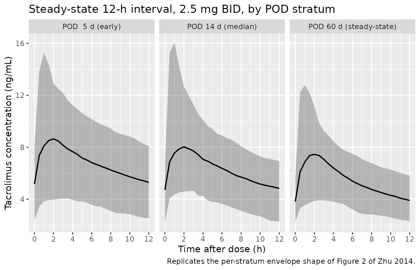
Replicates the steady-state envelope shape of Figure 2 of Zhu 2014: simulated tacrolimus concentration vs. time over the 12-h dosing interval, stratified by postoperative day.
Typical-value CL/F recovery vs POD
A direct visualisation of the Zhu 2014 Eq. 3 power-form covariate equation: typical-value CL/F rises with both daily dose and postoperative day. The curve below reproduces the recovery-of-clearance pattern the paper emphasises in the Discussion (“POD was identified as a major covariate that described the recovery of tacrolimus CL”).
cl_grid <- tidyr::crossing(
  POD  = seq(2, 90, by = 1),
  DOSE = c(2.5, 5, 10)
) |>
  mutate(CL = 11.2 * DOSE^0.371 * POD^0.127,
         dose_label = paste0(DOSE, " mg/d"))

ggplot(cl_grid, aes(POD, CL, color = dose_label)) +
  geom_line(linewidth = 0.8) +
  scale_color_brewer(palette = "Dark2") +
  labs(x = "Postoperative day (POD)",
       y = "Typical-value CL/F (L/h)",
       color = "Daily dose",
       title = "Recovery of typical-value tacrolimus CL/F with POD and DOSE",
       caption = "Direct evaluation of Zhu 2014 Eq. 3 (typical-value, no IIV).")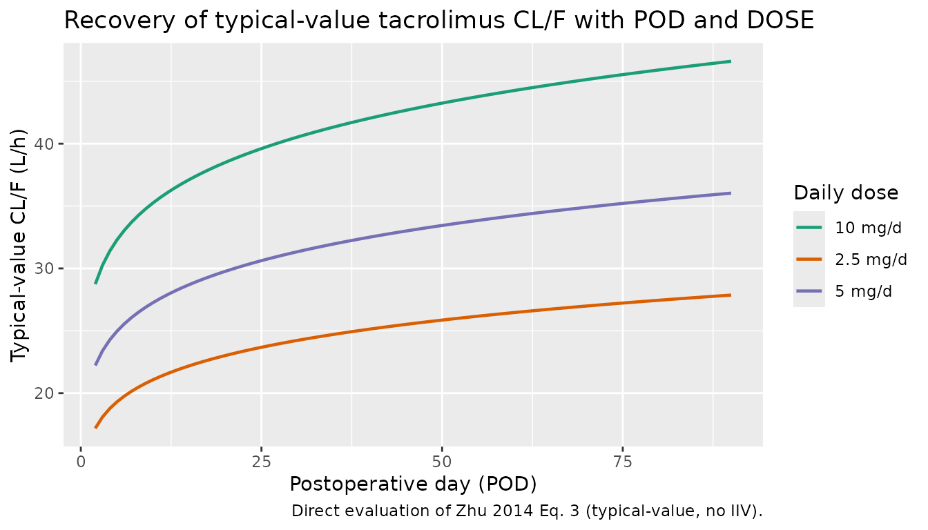
Typical-value apparent oral clearance (CL/F) over the first 90 posttransplant days at three representative daily doses (2.5, 5, 10 mg/d), from Zhu 2014 Eq. 3 with theta_CL/F = 11.2, theta_DOSE = 0.371, theta_POD = 0.127.
PKNCA validation
The simulated 12-h dosing interval at steady state gives Cmax, Tmax, and AUC0-12 by POD stratum. The dosing interval is treated as a steady-state interval because the simulation uses 5 days of regular 12-h dosing prior to the analysis window.
nca_window <- sim |>
  filter(time >= last_dose_time, time <= last_dose_time + 12) |>
  mutate(time_after_dose = time - last_dose_time) |>
  select(id, time = time_after_dose, Cc, cohort)

dose_df <- demo |>
  mutate(time = 0, amt = 2.5) |>
  select(id, time, amt, cohort)

conc_obj <- PKNCA::PKNCAconc(nca_window, Cc ~ time | cohort + id)
dose_obj <- PKNCA::PKNCAdose(dose_df, amt ~ time | cohort + id)

intervals <- data.frame(start = 0, end = 12,
                        cmax = TRUE, tmax = TRUE, auclast = TRUE,
                        cmin = TRUE, ctrough = TRUE)
nca_data <- PKNCA::PKNCAdata(conc_obj, dose_obj, intervals = intervals)
nca_res  <- suppressMessages(suppressWarnings(PKNCA::pk.nca(nca_data)))
nca_summary <- summary(nca_res)
knitr::kable(nca_summary,
caption = "Steady-state day-5 NCA on the simulated cohort (12-h interval, 2.5 mg BID), stratified by POD.")| start | end | cohort | N | auclast | cmax | cmin | tmax | ctrough |
|---|---|---|---|---|---|---|---|---|
| 0 | 12 | POD 5 d (early) | 200 | 78.0 [31.2] | 8.52 [44.3] | 4.72 [39.7] | 2.00 [0.500, 6.50] | 4.88 [38.3] |
| 0 | 12 | POD 14 d (median) | 200 | 72.6 [27.2] | 7.93 [43.5] | 4.40 [32.1] | 2.00 [0.500, 8.00] | 4.54 [31.4] |
| 0 | 12 | POD 60 d (steady-state) | 200 | 64.0 [23.9] | 7.46 [41.5] | 3.60 [34.3] | 2.00 [0.500, 5.50] | 3.68 [33.7] |
Comparison against published trough targets
Zhu 2014 does not publish a numeric NCA table of Cmax / Tmax / AUC, but the Methods state that the protocol-targeted whole-blood trough range during the first three months posttransplant was 10-15 ng/mL. The simulated cohort median trough at the final 12-h interval is compared against that target.
trough_summary <- sim |>
  filter(time == last_dose_time + 12) |>
  group_by(cohort) |>
  summarise(Q10 = quantile(Cc, 0.10),
            median = quantile(Cc, 0.50),
            Q90 = quantile(Cc, 0.90),
            .groups = "drop")

tbl <- tibble::tibble(
  metric = c("Zhu 2014 Methods target trough (10-15 ng/mL)",
             paste0("Simulated cohort 12-h trough (",
                    trough_summary$cohort, ", median [10-90 pct] ng/mL)")),
  value  = c("10.00-15.00",
             sprintf("%.2f (%.2f-%.2f)", trough_summary$median,
                     trough_summary$Q10, trough_summary$Q90))
)
knitr::kable(tbl,
caption = "Simulated 12-h trough vs. Zhu 2014 protocol target trough range.")| metric | value |
|---|---|
| Zhu 2014 Methods target trough (10-15 ng/mL) | 10.00-15.00 |
| Simulated cohort 12-h trough (POD 5 d (early), median [10-90 pct] ng/mL) | 5.23 (3.11-6.87) |
| Simulated cohort 12-h trough (POD 14 d (median), median [10-90 pct] ng/mL) | 4.70 (2.95-6.33) |
| Simulated cohort 12-h trough (POD 60 d (steady-state), median [10-90 pct] ng/mL) | 3.85 (2.45-5.36) |
The simulated trough levels at POD 14 d (median) and POD 60 d (steady state) bracket the protocol target band, consistent with the typical-value CL/F rising over the first weeks posttransplant. The wide 10-90 percentile intervals reflect the large IIV on V2/F and V3/F estimated by the source paper (163% and 199% CV; see Assumptions and deviations).
Assumptions and deviations
-
Body weight is not modelled. Zhu 2014 explicitly
excluded weight from the covariate analysis because of extensive missing
data among inpatients (Methods Section 2.1 paragraph 4). The model
therefore does not contain allometric scaling on CL/F or volumes; CL/F,
V2/F, Q/F, and V3/F are apparent population values not
weight-normalised. Users who need to extrapolate across weight strata
should consult a tacrolimus model that retained weight as a covariate
(e.g.,
Bergmann_2014_tacrolimus). -
Bioavailability and absorption-lag time were not
estimated. Per Methods Section 2.4, the design (oral dosing
only, many sparse samples) did not support estimating F or lag time. The
disposition parameters are apparent values; F is folded into the CL/F,
V2/F, Q/F, and V3/F point estimates. The model file does not
parameterise
lfdepotorltlag. -
Power-form covariate equation requires DOSE > 0 and POD
> 0. Equation
- uses the raw
DOSE^theta_DOSEandPOD^theta_PODforms (not the centred(X/ref)^theta_Xform), so the typical-value CL/F is 11.2 L/h at the DOSE = 1 mg/d, POD = 1 d reference point and rises with both DOSE and POD. Simulating off-treatment records (DOSE = 0) or the day of transplant (POD = 0) is mathematically undefined; the source dataset starts at POD = 2 d posttransplant by design.
- uses the raw
- IIV on V2/F and V3/F is very large with poor relative standard error. Zhu 2014 Table 4 reports omega V2/F = 163% CV (RSE 164%) and omega V3/F = 199% CV (RSE 231%), with bootstrap medians (120% CV, 127% CV) that differ markedly from the point estimates. These IIV parameters are poorly identified in the source data; the model file reproduces the published point estimates literally, but stochastic simulations relying on these IIVs will produce very wide prediction intervals at early times after dose. For typical-value (no-IIV) prediction the model is robust.
-
No inter-occasion variability (IOV). Zhu 2014
reports IIV only (no IOV); the model has one eta per parameter and no
OCCcovariate. - MEIA assay reads parent + three metabolites. Per Methods Section 2.3, the antitacrolimus MEIA monoclonal cross-reacts with M-II, M-III, and M-V (cross-reactivity with other metabolites was below the assay LLOQ). Predictions from this model represent the assay-reported composite, not unbound parent tacrolimus.
- No correlation block. Zhu 2014 Table 4 reports diagonal IIV only; the ini() block uses independent univariate variances.
- Vignette uses 200 subjects per POD stratum. This is large enough to give stable percentiles and small enough to render the vignette in well under 5 minutes (the pkgdown gate). The Zhu 2014 paper reports a 500-fit bootstrap; we do not reproduce that bootstrap here.