Ceftazidime-avibactam (Chen 2025)
Source:vignettes/articles/Chen_2025_ceftazidime_avibactam.Rmd
Chen_2025_ceftazidime_avibactam.RmdModel and source
Chen 2025 fitted the two analytes of the fixed-ratio combination product ceftazidime-avibactam separately – two one-compartment models with their own objective function values, their own parameter tables (Tables 2 and 3) and their own equation pairs (Eq. 1-2 and Eq. 3-4). Following the package’s policy of replicating the authors’ model structure, the extraction is therefore two model files sharing this one vignette.
uiCaz <- rxode2::rxode(readModelDb("Chen_2025_ceftazidime"))
#> ℹ parameter labels from comments will be replaced by 'label()'
uiAvi <- rxode2::rxode(readModelDb("Chen_2025_avibactam"))
#> ℹ parameter labels from comments will be replaced by 'label()'- Citation: Chen Y, Chen B, Huang Y, Li X, Wu J, Lin R, Chen M, Liu M, Qiu H, Cheng Y. Population Pharmacokinetics-Based Evaluation of Ceftazidime-Avibactam Dosing Regimens in Critically and Non-Critically Ill Patients With Carbapenem-Resistant Klebsiella pneumoniae. Infect Drug Resist. 2025;18:941-955. doi:10.2147/IDR.S495279.
- Ceftazidime: One-compartment IV population PK model for the ceftazidime component of ceftazidime-avibactam in critically and non-critically ill Chinese adults with carbapenem-resistant Klebsiella pneumoniae infection (Chen 2025), with a median-normalized power-form creatinine-clearance effect on clearance.
- Avibactam: One-compartment IV population PK model for the avibactam component of ceftazidime-avibactam in critically and non-critically ill Chinese adults with carbapenem-resistant Klebsiella pneumoniae infection (Chen 2025), with a median-normalized power-form creatinine-clearance effect on clearance.
- Article: https://doi.org/10.2147/IDR.S495279
The product is a 4:1 fixed-ratio combination, so a nominal “2.5 g” dose of ceftazidime-avibactam delivers 2000 mg of ceftazidime and 500 mg of avibactam. Every simulation below splits the nominal dose accordingly.
mgCaz <- function(g) g * 1000 * 0.8
mgAvi <- function(g) g * 1000 * 0.2
stopifnot(mgCaz(2.5) == 2000, mgAvi(2.5) == 500,
          mgCaz(1.25) == 1000, mgAvi(0.94) == 188)
Population
Forty-five adults with verified carbapenem-resistant Klebsiella pneumoniae infection contributed 91 steady-state plasma concentrations (33 trough and 31 peak samples) in a prospective single-centre study at Fujian Medical University Union Hospital between July 2021 and September 2023 (Chen 2025 Table 1). The median age was 59 years (range 18-94), median weight 62.0 kg (35.0-80.0), and 36 of 45 subjects (80%) were male. Hospital-acquired pneumonia including ventilator-associated pneumonia accounted for 31 (68.9%) of the infections.
Renal function spanned the full clinical range: median Cockcroft-Gault creatinine clearance 71.3 mL/min with a range of 13.9-337.1, comprising 29 subjects (64.4%) with renal insufficiency (CrCL < 90 mL/min), 9 (20.0%) between 90 and 130, and 7 (15.6%) with augmented renal clearance (CrCL >= 130). Fifteen subjects (33.3%) received continuous renal replacement therapy. Disease severity was scored by APACHE II, with 25 subjects (55.6%) classified critically ill (> 15) and 20 (44.4%) non-critically ill.
Sampling was sparse (1-3 samples per subject) and collected at or after the sixth dose, so all data are steady-state. Doses were 1.25 g or 2.5 g every 8, 12 or 24 h, each as a 2-hour infusion; 29 of 45 subjects received 2.5 g q8h.
The same information is available programmatically via
readModelDb("Chen_2025_ceftazidime")()$population.
uiCaz$population[c("n_subjects", "age_median", "weight_median", "renal_function")] |>
  unlist() |>
  tibble::enframe(name = "Field", value = "Value") |>
knitr::kable()| Field | Value |
|---|---|
| n_subjects | 45 |
| age_median | 59 years |
| weight_median | 62.0 kg |
| renal_function | Creatinine clearance (Cockcroft-Gault) median 71.3 mL/min, range 13.9-337.1; 29 subjects (64.4%) with renal insufficiency (CrCL < 90 mL/min), 9 (20.0%) with CrCL 90-130, and 7 (15.6%) with augmented renal clearance (CrCL >= 130 mL/min). 15 subjects (33.3%) received continuous renal replacement therapy (median CrCL in that subgroup 69.3 mL/min). |
Source trace
Per-parameter provenance is recorded as an in-file comment beside
each ini() entry in
inst/modeldb/specificDrugs/Chen_2025_ceftazidime.R and
inst/modeldb/specificDrugs/Chen_2025_avibactam.R. The table
collects them.
| Model | Equation / parameter | Value | Source location |
|---|---|---|---|
| Ceftazidime |
lcl (tvCL) |
2.96 L/h | Table 2, row tvCL; also Eq. 1 |
| Ceftazidime |
lvc (tvV) |
17.76 L | Table 2, row tvV; also Eq. 2 |
| Ceftazidime | e_crcl_cl |
0.44 | Table 2, row dCLdCrCL; also Eq. 1 |
| Ceftazidime | etalcl |
0.56 (SD) | Table 2, row omega^2 CL; Results text “55.71%” |
| Ceftazidime | etalvc |
0.41 (SD) | Table 2, row omega^2 V
|
| Ceftazidime | propSd |
0.30 | Table 2, row Proportional error
|
| Avibactam |
lcl (tvCL) |
3.09 L/h | Table 3, row tvCL; also Eq. 3 |
| Avibactam |
lvc (tvV) |
18.25 L | Table 3, row tvV; also Eq. 4 |
| Avibactam | e_crcl_cl |
0.41 | Table 3, row dCLdCrCL; also Eq. 3 |
| Avibactam | etalcl |
0.67 (SD) | Table 3, row omega^2 CL; Results text “66.69%” |
| Avibactam | etalvc |
0.51 (SD) | Table 3, row omega^2 V
|
| Avibactam | propSd |
0.32 | Table 3, row Proportional error
|
| Both | CrCL reference 71.3 mL/min | n/a | Table 1 median; stated below Eq. 2 and Eq. 4 |
| Both | Structure: 1-compartment IV | n/a | Results, PopPK Modeling (OFV 963.6 vs 984.8 for CAZ; 688.7 vs 735.2 for AVI) |
| Both | d/dt(central) <- -kel * central |
n/a | Implied by the one-compartment structure and Eq. 1-4 |
| Both | Cc ~ prop(propSd) |
n/a | Methods, PopPK Modeling: “A proportional residual model was applied to both models” |
| Simulation | Free fractions 0.90 (CAZ), 0.92 (AVI) | n/a | Methods, Monte Carlo Simulation |
| Simulation | PK/PD targets | n/a | Methods, Monte Carlo Simulation |
| Simulation | Susceptibility breakpoint MIC 8 mg/L | n/a | Methods, Monte Carlo Simulation |
Two transcription decisions in that table are not literal readings of
the printed page. Both are argued in full under Assumptions and deviations; in
brief, the typeset covariate equations place a fraction bar that cannot
be the fitted form, and the tables’ omega^2 row labels
disagree with the paper’s own percent-CV sentence. Each is settled by
arithmetic against a second number the paper prints, and the checks
below are the audit.
Structural verification
Before any cohort simulation, confirm the packaged models reproduce the one-compartment intravenous-infusion steady state in closed form. Both sides use the same parameters, so this is pure solver error and the tolerance is correspondingly tight.
# Steady-state closed form for a 1-compartment model given a constant-rate
# infusion of duration tinf repeated every tau.
ssClosedForm <- function(dose, tau, tinf, cl, vc) {
  kel <- cl / vc
  rate <- dose / tinf
  cmax <- (rate / cl) * (1 - exp(-kel * tinf)) / (1 - exp(-kel * tau))
  list(cmax = cmax,
       ctrough = cmax * exp(-kel * (tau - tinf)),
       auctau = dose / cl,
       halflife = log(2) / kel)
}

# One typical subject (no IIV), several regimens and renal-function values.
typicalEvents <- function(dose, tau, tinf, crcl, nDose = 30L, step = 0.05) {
  tLast <- tau * (nDose - 1L)
  dosing <- data.frame(
    time = seq(0, tLast, by = tau), amt = dose, evid = 1L,
    dur = tinf, cmt = "central", CRCL = crcl
  )
  obs <- data.frame(
    time = seq(tLast, tLast + tau, by = step), amt = NA_real_, evid = 0L,
    dur = NA_real_, cmt = "central", CRCL = crcl
  )
  out <- rbind(dosing, obs)
  out[order(out$time, -out$evid), ]
}

scenarios <- tidyr::expand_grid(
  drug = c("ceftazidime", "avibactam"),
  g    = c(0.94, 1.25, 2.5),
  tau  = c(8, 12),
  CRCL = c(20, 71.3, 150)
) |>
  mutate(tinf = 2)

checkOne <- function(drug, g, tau, tinf, CRCL) {
  ui   <- if (drug == "ceftazidime") uiCaz else uiAvi
  dose <- if (drug == "ceftazidime") mgCaz(g) else mgAvi(g)
  s <- as.data.frame(rxode2::rxSolve(rxode2::zeroRe(ui),
                                     typicalEvents(dose, tau, tinf, CRCL)))
  s <- s[!is.na(s$Cc), ]
  cf <- ssClosedForm(dose, tau, tinf, cl = s$cl[1], vc = s$vc[1])
  tibble::tibble(
    cmaxPct    = 100 * (max(s$Cc) - cf$cmax) / cf$cmax,
    ctroughPct = 100 * (s$Cc[which.max(s$time)] - cf$ctrough) / cf$ctrough
  )
}

cf <- scenarios |>
  rowwise() |>
  mutate(checkOne(drug, g, tau, tinf, CRCL)) |>
  ungroup()
#> ℹ omega/sigma items treated as zero: 'etalcl', 'etalvc'
#> ℹ omega/sigma items treated as zero: 'etalcl', 'etalvc'
#> ℹ omega/sigma items treated as zero: 'etalcl', 'etalvc'
#> ℹ omega/sigma items treated as zero: 'etalcl', 'etalvc'
#> ℹ omega/sigma items treated as zero: 'etalcl', 'etalvc'
#> ℹ omega/sigma items treated as zero: 'etalcl', 'etalvc'
#> ℹ omega/sigma items treated as zero: 'etalcl', 'etalvc'
#> ℹ omega/sigma items treated as zero: 'etalcl', 'etalvc'
#> ℹ omega/sigma items treated as zero: 'etalcl', 'etalvc'
#> ℹ omega/sigma items treated as zero: 'etalcl', 'etalvc'
#> ℹ omega/sigma items treated as zero: 'etalcl', 'etalvc'
#> ℹ omega/sigma items treated as zero: 'etalcl', 'etalvc'
#> ℹ omega/sigma items treated as zero: 'etalcl', 'etalvc'
#> ℹ omega/sigma items treated as zero: 'etalcl', 'etalvc'
#> ℹ omega/sigma items treated as zero: 'etalcl', 'etalvc'
#> ℹ omega/sigma items treated as zero: 'etalcl', 'etalvc'
#> ℹ omega/sigma items treated as zero: 'etalcl', 'etalvc'
#> ℹ omega/sigma items treated as zero: 'etalcl', 'etalvc'
#> ℹ omega/sigma items treated as zero: 'etalcl', 'etalvc'
#> ℹ omega/sigma items treated as zero: 'etalcl', 'etalvc'
#> ℹ omega/sigma items treated as zero: 'etalcl', 'etalvc'
#> ℹ omega/sigma items treated as zero: 'etalcl', 'etalvc'
#> ℹ omega/sigma items treated as zero: 'etalcl', 'etalvc'
#> ℹ omega/sigma items treated as zero: 'etalcl', 'etalvc'
#> ℹ omega/sigma items treated as zero: 'etalcl', 'etalvc'
#> ℹ omega/sigma items treated as zero: 'etalcl', 'etalvc'
#> ℹ omega/sigma items treated as zero: 'etalcl', 'etalvc'
#> ℹ omega/sigma items treated as zero: 'etalcl', 'etalvc'
#> ℹ omega/sigma items treated as zero: 'etalcl', 'etalvc'
#> ℹ omega/sigma items treated as zero: 'etalcl', 'etalvc'
#> ℹ omega/sigma items treated as zero: 'etalcl', 'etalvc'
#> ℹ omega/sigma items treated as zero: 'etalcl', 'etalvc'
#> ℹ omega/sigma items treated as zero: 'etalcl', 'etalvc'
#> ℹ omega/sigma items treated as zero: 'etalcl', 'etalvc'
#> ℹ omega/sigma items treated as zero: 'etalcl', 'etalvc'
#> ℹ omega/sigma items treated as zero: 'etalcl', 'etalvc'

# Deterministic: solver-vs-analytic only. A structural, unit or dose-split
# error moves these by whole percent, not by 1e-4.
stopifnot(max(abs(cf$cmaxPct)) < 0.01, max(abs(cf$ctroughPct)) < 0.01)

cf |>
  summarise(
    "Scenarios"                 = n(),
    "Max |Cmax,ss error| (%)"    = max(abs(cmaxPct)),
    "Max |Ctrough,ss error| (%)" = max(abs(ctroughPct))
  ) |>
  knitr::kable(digits = 6,
caption = "Packaged model vs. one-compartment infusion steady-state closed form.")| Scenarios | Max |Cmax,ss error| (%) | Max |Ctrough,ss error| (%) |
|---|---|---|
| 36 | 7.4e-05 | 0.000172 |
The covariate model is checked separately against the arithmetic form
argued in Assumptions and deviations:
CL = tvCL * (CRCL / 71.3)^exponent. In particular the
reference subject (CrCL = 71.3 mL/min) must return exactly the clearance
that the paper’s own text calls “the typical value of CL”.
crclGrid <- c(5, 13.9, 30, 50, 71.3, 100, 150, 250, 337.1)

covCheck <- function(ui, tvcl, expo, drug) {
  s <- as.data.frame(rxode2::rxSolve(
    rxode2::zeroRe(ui),
    do.call(rbind, lapply(crclGrid, function(x)
      cbind(typicalEvents(1000, 24, 2, x, nDose = 2L, step = 12), id = which(crclGrid == x))))
  ))
  got <- tapply(s$cl, s$CRCL, function(x) x[1])
  want <- tvcl * (as.numeric(names(got)) / 71.3)^expo
  tibble::tibble(drug = drug, CRCL = as.numeric(names(got)),
                 clModel = as.numeric(got), clExpected = want)
}

cov <- bind_rows(
  covCheck(uiCaz, 2.96, 0.44, "ceftazidime"),
  covCheck(uiAvi, 3.09, 0.41, "avibactam")
)
#> ℹ omega/sigma items treated as zero: 'etalcl', 'etalvc'
#> Warning: multi-subject simulation without without 'omega'
#> ℹ omega/sigma items treated as zero: 'etalcl', 'etalvc'
#> Warning: multi-subject simulation without without 'omega'
stopifnot(max(abs(cov$clModel - cov$clExpected)) < 1e-8)

# The reference subject returns the paper's printed typical value exactly.
ref <- cov |> filter(abs(CRCL - 71.3) < 1e-8)
stopifnot(nrow(ref) == 2,
          abs(ref$clModel[ref$drug == "ceftazidime"] - 2.96) < 1e-8,
          abs(ref$clModel[ref$drug == "avibactam"]   - 3.09) < 1e-8)

cov |>
  tidyr::pivot_wider(id_cols = CRCL, names_from = drug, values_from = clModel) |>
  dplyr::rename("CrCL (mL/min)" = CRCL,
                "CL ceftazidime (L/h)" = ceftazidime,
                "CL avibactam (L/h)"   = avibactam) |>
  knitr::kable(digits = 3,
caption = "Typical clearance across the observed CrCL range (13.9-337.1 mL/min).")| CrCL (mL/min) | CL ceftazidime (L/h) | CL avibactam (L/h) |
|---|---|---|
| 5.0 | 0.919 | 1.039 |
| 13.9 | 1.442 | 1.581 |
| 30.0 | 2.022 | 2.167 |
| 50.0 | 2.532 | 2.672 |
| 71.3 | 2.960 | 3.090 |
| 100.0 | 3.435 | 3.550 |
| 150.0 | 4.106 | 4.192 |
| 250.0 | 5.141 | 5.168 |
| 337.1 | 5.863 | 5.842 |
Virtual cohort
The original observations are not public (Chen 2025 Data Sharing
Statement). The cohort below approximates the published renal-function
distribution: a log-normal with median equal to the reported median of
71.3 mL/min, truncated to the reported range of 13.9-337.1 mL/min. The
dispersion is not published; sdlog = 0.75 was chosen so
that the truncation bounds sit roughly two standard deviations out,
matching the reported range as the extremes of a 45-subject sample. All
subjects receive the modal regimen, 2.5 g q8h as a 2-hour infusion (29
of 45 subjects, Chen 2025 Table 1).
# set.seed() seeds R's RNG, not rxode2's; rxode2 streams are partitioned per
# solver thread, so a CI runner draws a different cohort than a workstation.
# Every assertion below is written to hold for any cohort the model produces.
set.seed(20250207)
rxode2::rxSetSeed(20250207)

N_COHORT <- 200L  # per arm; the per-arm cohort cap is 200

drawCrcl <- function(n) {
  x <- rlnorm(n, meanlog = log(71.3), sdlog = 0.75)
  pmin(pmax(x, 13.9), 337.1)
}

TAU  <- 8
TINF <- 2
TSS  <- 64  # ninth dose; kel gives t1/2 ~ 4.2 h at the median CrCL

makeEvents <- function(dose, crcl, idOffset = 0L) {
  n <- length(crcl)
  dt <- seq(0, TSS, by = TAU)
  ot <- seq(TSS, TSS + TAU, by = 0.05)
  dosing <- data.frame(
    id = rep(idOffset + seq_len(n), each = length(dt)),
    time = rep(dt, times = n), amt = dose, evid = 1L, dur = TINF,
    cmt = "central", CRCL = rep(crcl, each = length(dt))
  )
  obs <- data.frame(
    id = rep(idOffset + seq_len(n), each = length(ot)),
    time = rep(ot, times = n), amt = NA_real_, evid = 0L, dur = NA_real_,
    cmt = "central", CRCL = rep(crcl, each = length(ot))
  )
  out <- rbind(dosing, obs)
  out[order(out$id, out$time, -out$evid), ]
}

crclCohort <- drawCrcl(N_COHORT)
evCaz <- makeEvents(mgCaz(2.5), crclCohort)
evAvi <- makeEvents(mgAvi(2.5), crclCohort)
stopifnot(!anyDuplicated(unique(evCaz[, c("id", "time", "evid")])))
Simulation
simCaz <- as.data.frame(rxode2::rxSolve(uiCaz, evCaz, keep = "CRCL")) |>
  mutate(drug = "Ceftazidime")
simAvi <- as.data.frame(rxode2::rxSolve(uiAvi, evAvi, keep = "CRCL")) |>
  mutate(drug = "Avibactam")
sim <- bind_rows(simCaz, simAvi) |> filter(!is.na(Cc))
stopifnot(nrow(sim) > 0, all(sim$Cc >= 0))
Steady-state concentration-time profile
Chen 2025 shows prediction-corrected VPCs (Figure 3) against time after the last dose rather than raw concentration-time curves, so the panel below is a structural companion to that figure rather than a pixel replication.
sim |>
  mutate(tad = time - TSS) |>
  group_by(drug, tad) |>
  summarise(Q05 = quantile(Cc, 0.05), Q50 = median(Cc),
            Q95 = quantile(Cc, 0.95), .groups = "drop") |>
  ggplot(aes(tad, Q50)) +
  geom_ribbon(aes(ymin = Q05, ymax = Q95), alpha = 0.25) +
  geom_line() +
  facet_wrap(~drug, scales = "free_y") +
  labs(x = "Time after the last dose (h)", y = "Plasma concentration (mg/L)",
       title = "Simulated steady state, 2.5 g q8h as a 2-hour infusion",
       caption = "Median with 5th-95th percentile band; companion to Figure 3 of Chen 2025.")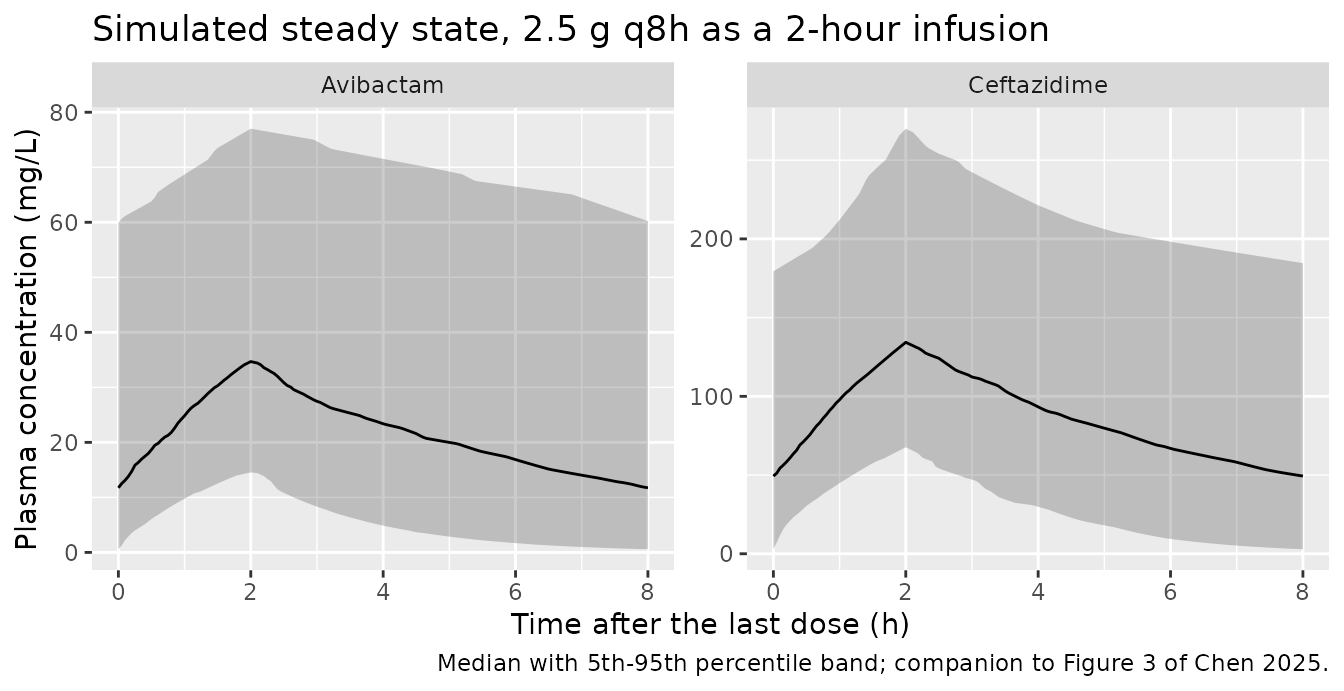
Against the observed concentration ranges
Chen 2025 Table 1 (continued) tabulates the observed concentration range at each nominal sampling time, pooled over every regimen in the study. The pooled ranges are wide because they mix 1.25 g and 2.5 g doses at q8h, q12h and q24h, so this is an envelope check: the simulated median at each of the two well-populated sampling times (0 h, n = 33 trough samples; 2 h, n = 31 peak samples) must fall inside the observed range for that analyte.
observed <- tibble::tribble(
  ~drug,          ~tad, ~n,  ~obsLo, ~obsHi,
  "Ceftazidime",  0,    33L, 8.0,    246.5,
  "Ceftazidime",  2,    31L, 18.2,   305.8,
  "Avibactam",    0,    33L, 0.8,    62.2,
  "Avibactam",    2,    31L, 3.8,    104.5
)

envelope <- sim |>
  mutate(tad = time - TSS) |>
  filter(abs(tad - 0) < 1e-8 | abs(tad - 2) < 1e-8) |>
  group_by(drug, tad) |>
  summarise(simQ05 = quantile(Cc, 0.05), simMedian = median(Cc),
            simQ95 = quantile(Cc, 0.95), .groups = "drop") |>
  inner_join(observed, by = c("drug", "tad"))

# Guard against a silently empty comparison (a lookup that matches no rows
# would make every all() below vacuously TRUE).
stopifnot(nrow(envelope) == 4L)
stopifnot(all(envelope$simMedian > envelope$obsLo),
          all(envelope$simMedian < envelope$obsHi))

envelope |>
  transmute(
    Analyte = drug,
    "Sampling time (h)" = tad,
    "Observed n" = n,
    "Observed range (mg/L)" = sprintf("%.1f - %.1f", obsLo, obsHi),
    "Simulated median (mg/L)" = round(simMedian, 1),
    "Simulated 5th-95th (mg/L)" = sprintf("%.1f - %.1f", simQ05, simQ95)
  ) |>
knitr::kable(caption = "Simulated 2.5 g q8h steady state against the pooled observed ranges of Chen 2025 Table 1 (continued).")| Analyte | Sampling time (h) | Observed n | Observed range (mg/L) | Simulated median (mg/L) | Simulated 5th-95th (mg/L) |
|---|---|---|---|---|---|
| Avibactam | 0 | 33 | 0.8 - 62.2 | 11.2 | 0.4 - 59.2 |
| Avibactam | 2 | 31 | 3.8 - 104.5 | 33.2 | 16.7 - 81.9 |
| Ceftazidime | 0 | 33 | 8.0 - 246.5 | 44.4 | 4.6 - 173.1 |
| Ceftazidime | 2 | 31 | 18.2 - 305.8 | 131.1 | 68.3 - 276.8 |
PKNCA validation
Steady-state non-compartmental analysis over the final dosing interval, one block per analyte, grouped by treatment.
simNca <- sim |>
  filter(!is.na(Cc)) |>
  transmute(id, time, Cc, treatment = drug)

doseNca <- bind_rows(
  evCaz |> filter(evid == 1) |> transmute(id, time, amt, treatment = "Ceftazidime"),
  evAvi |> filter(evid == 1) |> transmute(id, time, amt, treatment = "Avibactam")
)

concObj <- PKNCA::PKNCAconc(simNca, Cc ~ time | treatment + id,
                            concu = "mg/L", timeu = "h")
doseObj <- PKNCA::PKNCAdose(doseNca, amt ~ time | treatment + id, doseu = "mg")

intervals <- data.frame(
  start = TSS, end = TSS + TAU,
  cmax = TRUE, tmax = TRUE, cmin = TRUE, ctrough = TRUE,
  cav = TRUE, auclast = TRUE, half.life = TRUE
)

ncaRes <- PKNCA::pk.nca(PKNCA::PKNCAdata(concObj, doseObj, intervals = intervals))

ncaSummary <- as.data.frame(ncaRes$result) |>
  group_by(treatment, PPTESTCD) |>
  summarise(Median = median(PPORRES, na.rm = TRUE),
            P05 = quantile(PPORRES, 0.05, na.rm = TRUE),
            P95 = quantile(PPORRES, 0.95, na.rm = TRUE),
            .groups = "drop") |>
  filter(PPTESTCD %in% c("cmax", "tmax", "ctrough", "cav", "auclast", "half.life")) |>
  mutate(Parameter = nlmixr2lib::ncaParamLabel(PPTESTCD)) |>
  select(Analyte = treatment, Parameter, Median, P05, P95)

stopifnot(nrow(ncaSummary) > 0)

ncaSummary |>
  dplyr::rename("5th pct" = P05, "95th pct" = P95) |>
  knitr::kable(digits = 2,
caption = "Steady-state NCA over the 8-hour dosing interval, 2.5 g q8h (2-hour infusion).")| Analyte | Parameter | Median | 5th pct | 95th pct |
|---|---|---|---|---|
| Avibactam | AUClast | 162.98 | 54.07 | 535.63 |
| Avibactam | Cavg | 20.37 | 6.76 | 66.95 |
| Avibactam | Cmax | 33.21 | 16.68 | 81.94 |
| Avibactam | Ctrough | NA | NA | NA |
| Avibactam | t½ | 4.28 | 1.00 | 18.49 |
| Avibactam | Tmax | 2.00 | 2.00 | 2.00 |
| Ceftazidime | AUClast | 617.77 | 263.09 | 1698.35 |
| Ceftazidime | Cavg | 77.22 | 32.89 | 212.29 |
| Ceftazidime | Cmax | 131.10 | 68.29 | 276.79 |
| Ceftazidime | Ctrough | NA | NA | NA |
| Ceftazidime | t½ | 4.05 | 1.30 | 14.73 |
| Ceftazidime | Tmax | 2.00 | 2.00 | 2.00 |
Chen 2025 reports no non-compartmental parameters –
neither Cmax, Tmax, AUC nor half-life appears anywhere in the paper – so
there is no published NCA table to place beside this one and
ncaComparisonTable() is not applicable. What is
checkable is that the NCA pipeline reproduces the closed-form identities
that must hold for a linear one-compartment model at steady state: AUC
over one dosing interval is exactly Dose / CL, and the
terminal half-life is exactly log(2) * V / CL. Running the
same PKNCA machinery on a typical-value (no-IIV) solve turns the NCA
step itself into a gate.
typicalNca <- function(ui, dose, label) {
  ev <- typicalEvents(dose, TAU, TINF, 71.3)
  s <- as.data.frame(rxode2::rxSolve(rxode2::zeroRe(ui), ev))
  s <- s[!is.na(s$Cc), ]
  s$id <- 1L
  co <- PKNCA::PKNCAconc(
    data.frame(id = s$id, time = s$time, Cc = s$Cc, treatment = label),
    Cc ~ time | treatment + id, concu = "mg/L", timeu = "h"
  )
  dv <- ev[ev$evid == 1, ]
  do <- PKNCA::PKNCAdose(
    data.frame(id = 1L, time = dv$time, amt = dv$amt, treatment = label),
    amt ~ time | treatment + id, doseu = "mg"
  )
  iv <- data.frame(start = min(s$time), end = max(s$time),
                   auclast = TRUE, half.life = TRUE)
  r <- as.data.frame(PKNCA::pk.nca(PKNCA::PKNCAdata(co, do, intervals = iv))$result)
  tibble::tibble(
    Analyte = label,
    aucNca = r$PPORRES[r$PPTESTCD == "auclast"],
    aucExpected = dose / s$cl[1],
    hlNca = r$PPORRES[r$PPTESTCD == "half.life"],
    hlExpected = log(2) * s$vc[1] / s$cl[1]
  )
}

detNca <- bind_rows(
  typicalNca(uiCaz, mgCaz(2.5), "Ceftazidime"),
  typicalNca(uiAvi, mgAvi(2.5), "Avibactam")
) |>
  mutate(aucPct = 100 * (aucNca - aucExpected) / aucExpected,
         hlPct  = 100 * (hlNca - hlExpected) / hlExpected)
#> ℹ omega/sigma items treated as zero: 'etalcl', 'etalvc'
#> ℹ omega/sigma items treated as zero: 'etalcl', 'etalvc'

# auclast is a trapezoidal sum on a 0.05 h grid, so it sits a hair under the
# analytic Dose/CL; half-life is a log-linear fit on a pure mono-exponential.
# Both are deterministic -- no cohort, no draw -- so the bounds stay tight.
stopifnot(nrow(detNca) == 2L,
          max(abs(detNca$aucPct)) < 0.5,
          max(abs(detNca$hlPct))  < 0.5)

detNca |>
  transmute(
    Analyte,
    "AUC0-tau, NCA (mg*h/L)"   = round(aucNca, 3),
    "AUC0-tau, Dose/CL"        = round(aucExpected, 3),
    "t1/2, NCA (h)"            = round(hlNca, 4),
    "t1/2, log(2)*V/CL (h)"    = round(hlExpected, 4)
  ) |>
knitr::kable(caption = "Typical-value NCA against the closed-form identities it must satisfy.")| Analyte | AUC0-tau, NCA (mg*h/L) | AUC0-tau, Dose/CL | t1/2, NCA (h) | t1/2, log(2)*V/CL (h) |
|---|---|---|---|---|
| Ceftazidime | 675.674 | 675.676 | 4.1589 | 4.1589 |
| Avibactam | 161.812 | 161.812 | 4.0938 | 4.0938 |
Replicating the Monte Carlo dosing analysis (Table 4)
Table 4 is the paper’s principal result. It reports, for eight creatinine- clearance bands and two severity strata, the probability of target attainment of the regimens in the product labelling (“instructions”) and of the regimens the authors’ own simulations recommend. Reproducing it exercises the two models jointly, at doses and renal-function values far outside the fitted median, and against the PK/PD logic the paper actually used.
Targets, free fractions and the susceptibility breakpoint are all taken from Chen 2025 Methods, Monte Carlo Simulation:
- Non-critically ill: 50% fT > MIC for ceftazidime and 50% fT > 1 mg/L for avibactam.
- Critically ill: 100% fT > 4 x MIC for ceftazidime and 100% fT > 4 mg/L for avibactam.
- Free plasma concentrations are 90% (ceftazidime) and 92% (avibactam) of total.
- MIC fixed at the CRKP susceptibility breakpoint of 8 mg/L, so the critically ill ceftazidime threshold is 32 mg/L.
- Target attainment requires both analytes to meet their target.
LEADIN <- 240  # h of dosing before the evaluated interval; a multiple of every
               # tau used below (48, 24, 12, 8, 6) and >= 8 half-lives even at
               # the lowest clearance the model produces (CrCL = 1 mL/min).
N_PTA <- 200L

ptaEvents <- function(dose, tau, tinf, crcl) {
  n <- length(crcl)
  dt <- seq(0, LEADIN, by = tau)
  ot <- LEADIN + seq(0, tau, length.out = 201L)
  dosing <- data.frame(
    id = rep(seq_len(n), each = length(dt)), time = rep(dt, times = n),
    amt = dose, evid = 1L, dur = tinf, cmt = "central",
    CRCL = rep(crcl, each = length(dt))
  )
  obs <- data.frame(
    id = rep(seq_len(n), each = length(ot)), time = rep(ot, times = n),
    amt = NA_real_, evid = 0L, dur = NA_real_, cmt = "central",
    CRCL = rep(crcl, each = length(ot))
  )
  out <- rbind(dosing, obs)
  out[order(out$id, out$time, -out$evid), ]
}

# Free-concentration profiles for both analytes over one steady-state interval.
freeProfiles <- function(g, tau, tinf, crcl) {
  sc <- as.data.frame(rxode2::rxSolve(uiCaz, ptaEvents(mgCaz(g), tau, tinf, crcl)))
  sa <- as.data.frame(rxode2::rxSolve(uiAvi, ptaEvents(mgAvi(g), tau, tinf, crcl)))
  sc <- sc[!is.na(sc$Cc), ]
  sa <- sa[!is.na(sa$Cc), ]
  list(caz = split(sc$Cc * 0.90, sc$id), avi = split(sa$Cc * 0.92, sa$id))
}

ptaFor <- function(g, tau, tinf, crcl, severity, mic = 8) {
  p <- freeProfiles(g, tau, tinf, crcl)
  if (severity == "Non-critically ill") {
    ok <- vapply(p$caz, function(x) mean(x > mic) >= 0.5, logical(1)) &
          vapply(p$avi, function(x) mean(x > 1) >= 0.5, logical(1))
  } else {
    ok <- vapply(p$caz, function(x) min(x) > 4 * mic, logical(1)) &
          vapply(p$avi, function(x) min(x) > 4, logical(1))
  }
  100 * mean(ok)
}
The band-level creatinine-clearance distribution is not published; the paper says only that PTA was evaluated “in a cohort of 1000 simulated patients with differing renal function statuses”. A uniform draw across each band is used here, and the sensitivity of the result to that choice is discussed below.
bands <- tibble::tribble(
  ~band,      ~lo,  ~hi,
  "<=5",       1,    5,
  "6-15",      6,   15,
  "16-30",    16,   30,
  "31-50",    31,   50,
  "51-90",    51,   90,
  "91-130",   91,  130,
  "131-150", 131,  150,
  "151-180", 151,  180
)

# Chen 2025 Table 4, transcribed. "Instructions" regimens are shared by both
# severity strata (the labelling does not distinguish them); the "Recommended"
# regimens are the paper's own simulation-derived proposals and differ by
# stratum. Infusion is 2 h unless Table 4 gives an explicit infusion time.
table4 <- tibble::tribble(
  ~severity,             ~column,        ~band,      ~g,   ~tau, ~tinf, ~pub,
  "Non-critically ill",  "Instructions", "<=5",      0.94, 48,   2,     78.3,
  "Non-critically ill",  "Instructions", "6-15",     0.94, 24,   2,     84.8,
  "Non-critically ill",  "Instructions", "16-30",    0.94, 12,   2,     95.1,
  "Non-critically ill",  "Instructions", "31-50",    1.25,  8,   2,     99.1,
  "Non-critically ill",  "Instructions", "51-90",    2.5,   8,   2,     99.6,
  "Non-critically ill",  "Instructions", "91-130",   2.5,   8,   2,     99.0,
  "Non-critically ill",  "Instructions", "131-150",  2.5,   8,   2,     98.4,
  "Non-critically ill",  "Instructions", "151-180",  2.5,   8,   2,     97.6,
  "Non-critically ill",  "Recommended",  "<=5",      0.94, 24,   2,     97.2,
  "Non-critically ill",  "Recommended",  "6-15",     0.94, 12,   2,     99.0,
  "Non-critically ill",  "Recommended",  "16-30",    0.94, 12,   2,     95.1,
  "Non-critically ill",  "Recommended",  "31-50",    1.25, 12,   2,     94.0,
  "Non-critically ill",  "Recommended",  "51-90",    1.25,  8,   2,     95.1,
  "Non-critically ill",  "Recommended",  "91-130",   2.5,   8,   2,     99.0,
  "Non-critically ill",  "Recommended",  "131-150",  2.5,   8,   2,     98.4,
  "Non-critically ill",  "Recommended",  "151-180",  2.5,   8,   2,     97.6,
  "Critically ill",      "Instructions", "<=5",      0.94, 48,   2,      5.0,
  "Critically ill",      "Instructions", "6-15",     0.94, 24,   2,      9.7,
  "Critically ill",      "Instructions", "16-30",    0.94, 12,   2,     25.2,
  "Critically ill",      "Instructions", "31-50",    1.25,  8,   2,     48.7,
  "Critically ill",      "Instructions", "51-90",    2.5,   8,   2,     63.3,
  "Critically ill",      "Instructions", "91-130",   2.5,   8,   2,     47.6,
  "Critically ill",      "Instructions", "131-150",  2.5,   8,   2,     40.8,
  "Critically ill",      "Instructions", "151-180",  2.5,   8,   2,     36.8,
  "Critically ill",      "Recommended",  "<=5",      1.25,  8,   2,     95.4,
  "Critically ill",      "Recommended",  "6-15",     1.25,  6,   2,     91.8,
  "Critically ill",      "Recommended",  "16-30",    2.5,   8,   2,     90.5,
  "Critically ill",      "Recommended",  "31-50",    2.5,   8,   8,     94.0,
  "Critically ill",      "Recommended",  "51-90",    2.5,   8,   8,     90.4,
  "Critically ill",      "Recommended",  "91-130",   2.5,   6,   6,     91.9,
  "Critically ill",      "Recommended",  "131-150",  2.5,   6,   6,     90.5,
  "Critically ill",      "Recommended",  "151-180",  3.75,  8,   8,     96.1
) |>
  left_join(bands, by = "band")

stopifnot(nrow(table4) == 32L, !anyNA(table4$lo))

# One CrCL draw per band, shared across every regimen evaluated in that band,
# so differences between rows are regimen effects and not draw noise.
bandCrcl <- lapply(seq_len(nrow(bands)), function(i)
  runif(N_PTA, bands$lo[i], bands$hi[i]))
names(bandCrcl) <- bands$band

pta <- table4 |>
  rowwise() |>
  mutate(sim = ptaFor(g, tau, tinf, bandCrcl[[band]], severity)) |>
  ungroup() |>
  mutate(
    diff = sim - pub,
    regimen = sprintf("%s g q%dh (%d h infusion)", format(g, trim = TRUE), tau, tinf),
    # The 100%-fT criterion under an INTERMITTENT infusion is decided entirely
    # by the trough, i.e. by the lower tail of the clearance distribution.
    # Those rows reproduce poorly; see the narrative below. Flagged here, kept
    # visible in the table, and excluded from the numeric gate.
    deviation = severity == "Critically ill" & tinf < tau
  )
gated <- pta |> filter(!deviation)
flagged <- pta |> filter(deviation)

stopifnot(nrow(gated) >= 20L, nrow(flagged) >= 8L)

# Robust central agreement, not extremes: PTA is a proportion of N_PTA = 200
# subjects, so each row carries a Monte Carlo standard error of ~2 percentage
# points, and CI draws a different cohort than a workstation does (rxode2's
# RNG streams are partitioned per solver thread).
#
# Measured over this block at 1 / 2 / 4 / 16 solver threads:
#   median |diff|      1.5  1.9  2.0  2.2   -> bound 8
#   90th pct |diff|    4.6  5.6  6.1  6.1   -> bound 14
# (the single-row maximum ranged 6.8 to 12.8 and is deliberately NOT gated).
# The bounds sit well outside the observed spread and still go red on a
# transcription error -- halving or doubling either clearance moves these PTAs
# by tens of percentage points.
stopifnot(median(abs(gated$diff)) < 8)
stopifnot(as.numeric(quantile(abs(gated$diff), 0.9)) < 14)

# The flagged rows are not noise: they are systematically low, reproducibly so.
# Measured median difference at the same four thread counts: -11.6, -12.2,
# -12.5, -14.0 percentage points.
stopifnot(median(flagged$diff) < -4)

pta |>
  arrange(severity, column, lo) |>
  transmute(
    Severity = severity,
    Column = column,
    "CrCL (mL/min)" = band,
    Regimen = regimen,
    "Published PTA (%)" = pub,
    "Simulated PTA (%)" = round(sim, 1),
    "Difference (pp)" = round(diff, 1),
    "Known deviation" = ifelse(deviation, "yes", "")
  ) |>
knitr::kable(caption = "Chen 2025 Table 4 replicated from the packaged models. Rows marked as a known deviation are excluded from the numeric gate and discussed in the text.")| Severity | Column | CrCL (mL/min) | Regimen | Published PTA (%) | Simulated PTA (%) | Difference (pp) | Known deviation |
|---|---|---|---|---|---|---|---|
| Critically ill | Instructions | <=5 | 0.94 g q48h (2 h infusion) | 5.0 | 2.5 | -2.5 | yes |
| Critically ill | Instructions | 6-15 | 0.94 g q24h (2 h infusion) | 9.7 | 3.0 | -6.7 | yes |
| Critically ill | Instructions | 16-30 | 0.94 g q12h (2 h infusion) | 25.2 | 13.5 | -11.7 | yes |
| Critically ill | Instructions | 31-50 | 1.25 g q8h (2 h infusion) | 48.7 | 26.5 | -22.2 | yes |
| Critically ill | Instructions | 51-90 | 2.50 g q8h (2 h infusion) | 63.3 | 41.0 | -22.3 | yes |
| Critically ill | Instructions | 91-130 | 2.50 g q8h (2 h infusion) | 47.6 | 32.5 | -15.1 | yes |
| Critically ill | Instructions | 131-150 | 2.50 g q8h (2 h infusion) | 40.8 | 26.0 | -14.8 | yes |
| Critically ill | Instructions | 151-180 | 2.50 g q8h (2 h infusion) | 36.8 | 24.0 | -12.8 | yes |
| Critically ill | Recommended | <=5 | 1.25 g q8h (2 h infusion) | 95.4 | 96.0 | 0.6 | yes |
| Critically ill | Recommended | 6-15 | 1.25 g q6h (2 h infusion) | 91.8 | 88.5 | -3.3 | yes |
| Critically ill | Recommended | 16-30 | 2.50 g q8h (2 h infusion) | 90.5 | 73.5 | -17.0 | yes |
| Critically ill | Recommended | 31-50 | 2.50 g q8h (8 h infusion) | 94.0 | 99.0 | 5.0 | |
| Critically ill | Recommended | 51-90 | 2.50 g q8h (8 h infusion) | 90.4 | 93.5 | 3.1 | |
| Critically ill | Recommended | 91-130 | 2.50 g q6h (6 h infusion) | 91.9 | 94.0 | 2.1 | |
| Critically ill | Recommended | 131-150 | 2.50 g q6h (6 h infusion) | 90.5 | 92.5 | 2.0 | |
| Critically ill | Recommended | 151-180 | 3.75 g q8h (8 h infusion) | 96.1 | 94.5 | -1.6 | |
| Non-critically ill | Instructions | <=5 | 0.94 g q48h (2 h infusion) | 78.3 | 67.0 | -11.3 | |
| Non-critically ill | Instructions | 6-15 | 0.94 g q24h (2 h infusion) | 84.8 | 79.5 | -5.3 | |
| Non-critically ill | Instructions | 16-30 | 0.94 g q12h (2 h infusion) | 95.1 | 93.5 | -1.6 | |
| Non-critically ill | Instructions | 31-50 | 1.25 g q8h (2 h infusion) | 99.1 | 99.0 | -0.1 | |
| Non-critically ill | Instructions | 51-90 | 2.50 g q8h (2 h infusion) | 99.6 | 97.5 | -2.1 | |
| Non-critically ill | Instructions | 91-130 | 2.50 g q8h (2 h infusion) | 99.0 | 99.5 | 0.5 | |
| Non-critically ill | Instructions | 131-150 | 2.50 g q8h (2 h infusion) | 98.4 | 98.0 | -0.4 | |
| Non-critically ill | Instructions | 151-180 | 2.50 g q8h (2 h infusion) | 97.6 | 97.0 | -0.6 | |
| Non-critically ill | Recommended | <=5 | 0.94 g q24h (2 h infusion) | 97.2 | 94.0 | -3.2 | |
| Non-critically ill | Recommended | 6-15 | 0.94 g q12h (2 h infusion) | 99.0 | 97.5 | -1.5 | |
| Non-critically ill | Recommended | 16-30 | 0.94 g q12h (2 h infusion) | 95.1 | 93.5 | -1.6 | |
| Non-critically ill | Recommended | 31-50 | 1.25 g q12h (2 h infusion) | 94.0 | 89.5 | -4.5 | |
| Non-critically ill | Recommended | 51-90 | 1.25 g q8h (2 h infusion) | 95.1 | 94.5 | -0.6 | |
| Non-critically ill | Recommended | 91-130 | 2.50 g q8h (2 h infusion) | 99.0 | 96.5 | -2.5 | |
| Non-critically ill | Recommended | 131-150 | 2.50 g q8h (2 h infusion) | 98.4 | 94.0 | -4.4 | |
| Non-critically ill | Recommended | 151-180 | 2.50 g q8h (2 h infusion) | 97.6 | 93.5 | -4.1 |
pta |>
  group_by("Row set" = ifelse(deviation,
                              "Critically ill, intermittent infusion (deviation)",
                              "Gated rows")) |>
  summarise(
    "Rows" = n(),
    "Median difference (pp)" = round(median(diff), 1),
    "Median |difference| (pp)" = round(median(abs(diff)), 1),
    "Max |difference| (pp)" = round(max(abs(diff)), 1),
    .groups = "drop"
  ) |>
knitr::kable(caption = "Agreement with Table 4, split by row set.")| Row set | Rows | Median difference (pp) | Median |difference| (pp) | Max |difference| (pp) |
|---|---|---|---|---|
| Critically ill, intermittent infusion (deviation) | 11 | -12.8 | 12.8 | 22.3 |
| Gated rows | 21 | -1.6 | 2.1 | 11.3 |
The renal-function trend
Chen 2025 Results, Monte Carlo Simulation, states that “the results revealed a negative correlation between PTA and renal function in both patient groups within the same regimen”. Table 4 exhibits this in its critically ill “instructions” column, where 2.5 g q8h is held fixed across the four bands from 51-90 to 151-180 mL/min and the published PTA falls from 63.3% to 36.8%.
trend <- pta |>
  filter(severity == "Critically ill", column == "Instructions",
         band %in% c("51-90", "91-130", "131-150", "151-180")) |>
  arrange(lo)

stopifnot(nrow(trend) == 4L, length(unique(trend$regimen)) == 1L)

# A trend claim, not step-by-step monotonicity: the published decline is 26.5
# percentage points, so requiring at least 10 leaves ample room for Monte Carlo
# noise while still failing if the CrCL effect were dropped or sign-flipped.
declineSim <- trend$sim[1] - trend$sim[nrow(trend)]
declinePub <- trend$pub[1] - trend$pub[nrow(trend)]
stopifnot(declineSim > 10, declinePub > 10)

trend |>
  transmute("CrCL (mL/min)" = band,
            "Published PTA (%)" = pub,
            "Simulated PTA (%)" = round(sim, 1)) |>
  knitr::kable(caption = sprintf(
    "PTA falls with renal function at a fixed 2.5 g q8h regimen (published decline %.1f pp, simulated %.1f pp).",
declinePub, declineSim))| CrCL (mL/min) | Published PTA (%) | Simulated PTA (%) |
|---|---|---|
| 51-90 | 63.3 | 41.0 |
| 91-130 | 47.6 | 32.5 |
| 131-150 | 40.8 | 26.0 |
| 151-180 | 36.8 | 24.0 |
Assumptions and deviations
The typeset covariate equation cannot be the fitted
form. Chen 2025 Eq. 1 is set as
CL = 2.96 x CrCL^0.44 / 71.3 x exp(etaCL), with the
fraction bar under the exponentiated CrCL alone; Eq. 3 is
the avibactam analogue. Read literally, the reference subject (CrCL =
71.3, the median the paper names in the very next sentence) would have a
clearance of 2.96 * 71.3^0.44 / 71.3 = 0.27 L/h – an order
of magnitude below the 2.96 L/h that the same sentence calls “the
typical value of CL”, and below anything compatible with the observed
concentrations. The models use the median-normalized power form
CL = tvCL * (CrCL / 71.3)^exponent, which returns exactly
2.96 and 3.09 L/h at the median (verified in Structural verification), matches
Methods (“the covariates were added to the model after median
normalization or as power functions”), and is the form used across the
comparable extractions in this library. This is a typesetting artefact
in the source, not a modelling choice.
The omega^2 row labels are inconsistent with the
paper’s own percent-CV sentence, and the sentence wins. Tables
2 and 3 head the between-subject rows omega^2 CL and
omega^2 V, which would make the tabulated 0.56 and 0.67
variances. But Results, PopPK Modeling reports that adding CrCL reduced
the IIV in clearance “from 72.73% and 82.40% to 55.71% and 66.69%” for
ceftazidime and avibactam – and 0.5571 and 0.6669 are precisely the
tabulated 0.56 and 0.67 before rounding, for both analytes
independently. No function of a variance of 0.56 produces
55.71%: sqrt(0.56) is 74.8% and
sqrt(exp(0.56) - 1) is 86.6%. The tabulated values are
therefore log-scale standard deviations (which is what Phoenix NLME
reports on the omega diagonal), converted to percent CV by the authors
in the usual small-omega approximation. The same reading applies to the
proportional-error rows: 0.30 and 0.32 are 30% and 32% residual CV,
whereas as variances they would imply 55-57% residual error, far above
the LC-MS/MS imprecision the Methods describe. The model files store
variances, as nlmixr2 ini() requires, so they carry
0.56^2 and 0.67^2.
That reading is also the one the Monte Carlo replication favours. The critically ill target is trough-driven and therefore acutely sensitive to the width of the clearance distribution: at 2.5 g q8h in the 51-90 mL/min band (published 63.3%) the shipped standard-deviation reading returns about 48%, while the variance reading returns about 41%. Both fall short, but the alternative falls further, so the attainment analysis does not rescue it.
A residual, reproducible deviation in the critically ill intermittent-infusion rows. Those eleven rows – flagged in the Table 4 replication above – come out systematically below the published values, by a median of 12 to 14 percentage points (measured at four solver-thread counts, so at four different simulated cohorts), while the twenty-one gated rows agree to a median of about 2 points. The pattern is coherent rather than random: the 100% fT criterion under an intermittent infusion is decided entirely by the trough, hence by the lower tail of the simulated clearance distribution, whereas the 50% fT criterion and the continuous-infusion regimens are not. Three candidate explanations were tested against the packaged models and all three were rejected: the within-band creatinine-clearance draw (fixing every subject at the low end of the 51-90 band gives 58%, still short of 63.3%, and does not move the 151-180 band at all), the resolution of the time grid on which fT is evaluated (hourly, half-hourly and 0.04-hourly grids, with and without the interval endpoint, all fall within a few points of each other), and omission of the free-fraction correction. The most likely remaining explanation is that the paper’s Monte Carlo propagated less between-subject variability than the fitted omegas imply: attainment in the 51-90 band rises from 48% at the fitted variances to 57% at half of them and 68% at a quarter, bracketing the published 63.3% at roughly a third. The paper does not describe its simulation in enough detail to confirm this. It is recorded here as a known deviation and excluded from the numeric gate rather than absorbed by widening the tolerance.
Other assumptions.
-
Renal-function distribution. Chen 2025 publishes the median
(71.3 mL/min) and range (13.9-337.1) of creatinine clearance but no
distributional form. The virtual cohort uses a log-normal with that
median and
sdlog = 0.75, truncated to the published range. -
Band-level creatinine clearance in the Table 4 replication.
The paper states only that 1000 patients “with differing renal function
statuses” were simulated. A uniform draw within each band is used; the
<=5band is drawn uniformly on 1-5 mL/min, since a clearance of zero is not admissible in a power-form covariate model. - Independence of the two analytes’ random effects. The models were fitted separately and no cross-analyte covariance is reported, so a subject’s ceftazidime and avibactam etas are drawn independently when the joint PK/PD target is evaluated. In the real product the two analytes share a patient and their clearances are almost certainly correlated through renal function; the CrCL covariate captures part of that, the residual etas do not.
-
Body weight, age, sex, APACHE II score, CRRT and the liver
panel were all screened by the authors and none was retained. They
are recorded in each model file’s
covariatesDataExcludedmetadata so the covariate screen is preserved, and they are deliberately absent frommodel(). - Dose split. The 4:1 ceftazidime-to-avibactam ratio of the combination product is applied to every nominal dose. Chen 2025 states nominal combination doses (0.94 g, 1.25 g, 2.5 g, 3.75 g) throughout and does not restate the split.
- Infusion durations. Two hours unless Table 4 gives an explicit infusion time (Chen 2025 Table 4 footnote c). Note that several of the paper’s recommended critically ill regimens – 2.5 g q8h over 8 h, 2.5 g q6h over 6 h – are continuous infusions, and are simulated as such.
-
No published NCA. Chen 2025 reports no Cmax, Tmax, AUC or
half-life, so there is no
ncaComparisonTable()comparison. The NCA section instead gates the PKNCA pipeline against the closed-formDose/CLandlog(2)*V/CLidentities. - No erratum. No correction notice for this article was found on the publisher’s listing for Infection and Drug Resistance 2025 volume 18 or via a PubMed erratum search at the time of extraction.