Atezolizumab (Zeng 2026)
Source:vignettes/articles/Zeng_2026_atezolizumab.Rmd
Zeng_2026_atezolizumab.RmdProvenance: what this model is, and what it is not
Zeng et al. (2026) is a software benchmark, not a model-development paper. Its subject is a three-way comparison of NONMEM 7.5.1, RxODE and Pumas 2.5.1 running the same atezolizumab population PK model over the same virtual population, and its headline results are throughput numbers (observations simulated per second).
The extractable content is in the supplement, which contains the complete NONMEM control stream under the heading
“Atezolizumab Simulation Model: Duplicated from FDA CDER Clinical Pharmacology and Biopharmaceutics Review; 761041Orig1s000”
together with the equivalent RxODE rxode2({...}) model
object and Pumas @model block. All 17 $THETA
entries, all 4 $OMEGA entries and $SIGMA carry
FIX. Three consequences follow, and they shape this
vignette:
-
Every parameter in the nlmixr2lib model is wrapped in
fixed(). Nothing here was estimated from data; the values are the FDA review’s estimates, transcribed by the authors and held constant for simulation. - The primary source of the parameter values is the FDA CDER review of BLA 761041Orig1s000, which is not in nlmixr2lib. Zeng 2026 is the transcription source. If the FDA review is obtained later, this extraction should be re-checked against it.
- The validation targets are the paper’s own simulated exposures, not observed clinical data. That is unusually favourable rather than weak: the paper publishes its covariate-generation code with its random seed, and a supplementary table reports exposures with the random effects switched off, so the published numbers can be reproduced outright instead of merely bracketed.
mod <- rxode2::rxode(readModelDb("Zeng_2026_atezolizumab"))
#> ℹ parameter labels from comments will be replaced by 'label()'
mod$description
#> [1] "Two-compartment population PK model for intravenous atezolizumab (anti-PD-L1 IgG1) in patients with metastatic non-small cell lung cancer, with sigmoidal time-varying clearance (Zeng 2026): every fixed effect, variance and residual-error term is held FIXED for simulation, transcribed from the FDA CDER clinical pharmacology and biopharmaceutics review for BLA 761041Orig1s000. The source publication is a three-way software benchmark (NONMEM, RxODE, Pumas) whose supplement carries the complete NONMEM control stream plus the equivalent RxODE and Pumas model objects."
Population
pop <- mod$population
str(pop)
#> List of 11
#>  $ species       : chr "human"
#>  $ n_subjects    : num 1000
#>  $ n_studies     : num 1
#>  $ age_range     : chr "20-80 years"
#>  $ age_median    : chr "44.6-51 years across the three software implementations"
#>  $ weight_range  : chr "43.2-136 kg"
#>  $ weight_median : chr "79.6-83.2 kg across the three software implementations"
#>  $ sex_female_pct: num 51.2
#>  $ disease_state : chr "Metastatic non-small cell lung cancer (the underlying population PK model was developed in NSCLC patients per t"| __truncated__
#>  $ dose_range    : chr "840, 1200 or 1680 mg IV; standard 1200 mg q3w and three extended-interval regimens (2 loading cycles at 840 mg "| __truncated__
#>  $ notes         : chr "The 1000 subjects are a SIMULATED virtual population, not an estimation dataset: this model was not fitted to o"| __truncated__
The 1000 subjects are a simulated virtual population, not an estimation cohort. The underlying population PK model was developed in metastatic non-small cell lung cancer patients (FDA CDER review of BLA 761041Orig1s000).
Source trace
Every value in ini() and every non-trivial line of
model(), with the exact location it came from.
MOESM1 is the Zeng 2026 supplementary Word document;
“NONMEM” refers to its Atezolizumab Simulation Model
control stream.
source_trace <- tibble::tribble(
  ~Quantity,                       ~Value,        ~`Source location`,
  "CL (L/day)",                    "0.23",        "MOESM1 NONMEM $THETA(3)",
  "Vc (L)",                        "3.25",        "MOESM1 NONMEM $THETA(4)",
  "Q (L/day)",                     "0.603",       "MOESM1 NONMEM $THETA(5)",
  "Vp (L)",                        "2.88",        "MOESM1 NONMEM $THETA(6)",
  "cl_time_max (IMAX)",            "-0.193",      "MOESM1 NONMEM $THETA(15)",
  "cl_t50 (day)",             "62.8",        "MOESM1 NONMEM $THETA(16)",
  "cl_time_hill",                 "2.67",        "MOESM1 NONMEM $THETA(17)",
  "WT exponent on CL",             "0.668",       "MOESM1 NONMEM $THETA(7)",
  "ALB exponent on CL",            "-0.901",      "MOESM1 NONMEM $THETA(8)",
  "TUMSZ exponent on CL",          "0.116",       "MOESM1 NONMEM $THETA(9)",
  "ADA_POS factor on CL",          "1.158",       "MOESM1 NONMEM $THETA(10)",
  "WT exponent on Vc",             "0.533",       "MOESM1 NONMEM $THETA(11)",
  "ALB exponent on Vc",            "-0.345",      "MOESM1 NONMEM $THETA(12)",
  "SEXF factor on Vc",             "0.896",       "MOESM1 NONMEM $THETA(13)",
  "SEXF factor on Vp",             "0.707",       "MOESM1 NONMEM $THETA(14)",
  "IIV CL (variance)",             "0.069169",    "MOESM1 NONMEM $OMEGA ETA(1)",
  "IIV Vc (variance)",             "0.029584",    "MOESM1 NONMEM $OMEGA ETA(2)",
  "IIV Vp (variance)",             "0.123904",    "MOESM1 NONMEM $OMEGA ETA(3)",
  "IIV cl_time_max (variance)",    "0.804609",    "MOESM1 NONMEM $OMEGA ETA(4)",
  "Proportional residual SD",      "0.034",       "MOESM1 NONMEM $THETA(1), $ERROR W",
  "Additive residual SD (ug/mL)",  "18.1",        "MOESM1 NONMEM $THETA(2), $ERROR W",
  "Reference WT / ALB / TUMSZ",    "77 kg / 40 g/L / 63 mm", "MOESM1 NONMEM $PK",
  "2-compartment IV structure",    "ADVAN3 TRANS4", "MOESM1 NONMEM $SUBROUTINES",
  "CL(t) sigmoid form",            "CL * exp(IMAX * t^GMA / (T50^GMA + t^GMA))", "MOESM1 NONMEM $PK",
  "Residual error form",           "W = sqrt(prop^2 * IPRED^2 + add^2)", "MOESM1 NONMEM $ERROR",
  "Covariate distributions, seed", "seed 12345",  "MOESM1 population-generation code",
  "Dosing regimens",               "1200 q3w; 840 q2w x2 / 1200 q3w x2 / 1680 q4w x2 then 840 q6w x5",
  "Zeng 2026 Methods; Table 2; Figs. 1-3",
  "Realised cohort demographics",  "n = 1000",    "Zeng 2026 Table 1",
  "Published exposures (IIV on)",  "geometric mean (90% PI), n = 1000", "Zeng 2026 Table 2",
  "Published exposures (IIV off)", "Cmax 269.5, Cmin 72.4, weekly AUC 818.8, n = 100",
  "MOESM1 Supplemental Table 1"
)
knitr::kable(source_trace)| Quantity | Value | Source location |
|---|---|---|
| CL (L/day) | 0.23 | MOESM1 NONMEM $THETA(3) |
| Vc (L) | 3.25 | MOESM1 NONMEM $THETA(4) |
| Q (L/day) | 0.603 | MOESM1 NONMEM $THETA(5) |
| Vp (L) | 2.88 | MOESM1 NONMEM $THETA(6) |
| cl_time_max (IMAX) | -0.193 | MOESM1 NONMEM $THETA(15) |
| cl_t50 (day) | 62.8 | MOESM1 NONMEM $THETA(16) |
| cl_time_hill | 2.67 | MOESM1 NONMEM $THETA(17) |
| WT exponent on CL | 0.668 | MOESM1 NONMEM $THETA(7) |
| ALB exponent on CL | -0.901 | MOESM1 NONMEM $THETA(8) |
| TUMSZ exponent on CL | 0.116 | MOESM1 NONMEM $THETA(9) |
| ADA_POS factor on CL | 1.158 | MOESM1 NONMEM $THETA(10) |
| WT exponent on Vc | 0.533 | MOESM1 NONMEM $THETA(11) |
| ALB exponent on Vc | -0.345 | MOESM1 NONMEM $THETA(12) |
| SEXF factor on Vc | 0.896 | MOESM1 NONMEM $THETA(13) |
| SEXF factor on Vp | 0.707 | MOESM1 NONMEM $THETA(14) |
| IIV CL (variance) | 0.069169 | MOESM1 NONMEM $OMEGA ETA(1) |
| IIV Vc (variance) | 0.029584 | MOESM1 NONMEM $OMEGA ETA(2) |
| IIV Vp (variance) | 0.123904 | MOESM1 NONMEM $OMEGA ETA(3) |
| IIV cl_time_max (variance) | 0.804609 | MOESM1 NONMEM $OMEGA ETA(4) |
| Proportional residual SD | 0.034 | MOESM1 NONMEM $THETA(1), $ERROR W |
| Additive residual SD (ug/mL) | 18.1 | MOESM1 NONMEM $THETA(2), $ERROR W |
| Reference WT / ALB / TUMSZ | 77 kg / 40 g/L / 63 mm | MOESM1 NONMEM $PK |
| 2-compartment IV structure | ADVAN3 TRANS4 | MOESM1 NONMEM $SUBROUTINES |
| CL(t) sigmoid form | CL * exp(IMAX * t^GMA / (T50^GMA + t^GMA)) | MOESM1 NONMEM $PK |
| Residual error form | W = sqrt(prop^2 * IPRED^2 + add^2) | MOESM1 NONMEM $ERROR |
| Covariate distributions, seed | seed 12345 | MOESM1 population-generation code |
| Dosing regimens | 1200 q3w; 840 q2w x2 / 1200 q3w x2 / 1680 q4w x2 then 840 q6w x5 | Zeng 2026 Methods; Table 2; Figs. 1-3 |
| Realised cohort demographics | n = 1000 | Zeng 2026 Table 1 |
| Published exposures (IIV on) | geometric mean (90% PI), n = 1000 | Zeng 2026 Table 2 |
| Published exposures (IIV off) | Cmax 269.5, Cmin 72.4, weekly AUC 818.8, n = 100 | MOESM1 Supplemental Table 1 |
Time-scale reconciliation
The supplement states the model twice on two different time scales, which is what makes the day-scale reading of the NONMEM stream certain rather than inferred:
tibble::tibble(
  Parameter = c("CL", "Q", "T50"),
  `Pumas (hour scale)` = c(0.009583, 0.025125, 1507.1999),
  `x 24 or / 24` = c(0.009583 * 24, 0.025125 * 24, 1507.1999 / 24),
  `NONMEM / RxODE (day scale)` = c(0.23, 0.603, 62.8)
) |>
knitr::kable(digits = 5)| Parameter | Pumas (hour scale) | x 24 or / 24 | NONMEM / RxODE (day scale) |
|---|---|---|---|
| CL | 0.00958 | 0.22999 | 0.230 |
| Q | 0.02513 | 0.60300 | 0.603 |
| T50 | 1507.19990 | 62.80000 | 62.800 |
Virtual cohort
Reproduced verbatim from the supplement’s population-generation code, in the same statement order and with the same seed. Age is used only to generate body weight; it is not a covariate of the PK model.
make_cohort <- function(n, seed = 12345) {
  set.seed(seed)
  AGE <- round(runif(n, min = 20, max = 80))
  SEXF <- round(runif(n, min = 0, max = 1))
  BWf <- 65 + 0.75 * (AGE - 40) + rnorm(n, 0, sd = 3.5)
  BWm <- 85 + 0.75 * (AGE - 40) + rnorm(n, 0, sd = 10)
  data.frame(
    id      = seq_len(n),
    AGE     = AGE,
    SEXF    = SEXF,
    WT      = ifelse(SEXF == 1, BWf, BWm),
    ADA_POS = rbinom(n, 1, 0.4),
    ALB     = rnorm(n, 42, sd = 3.5),
    TUMSZ   = rlnorm(n, 4.2, sd = 0.7)
  )
}
cohort_1000 <- make_cohort(1000)
The generator reproduces the published cohort
Before trusting any exposure comparison, check the cohort itself. Zeng 2026 Table 1 reports the realised demographics of the n = 1000 virtual population for each software. Four of the five summaries match exactly.
cohort_check <- tibble::tibble(
  Summary = c("Female (%)", "ADA-positive (%)", "WT median (kg)",
              "ALB median (g/L)", "TUMSZ median (mm)"),
  Reproduced = c(100 * mean(cohort_1000$SEXF), 100 * mean(cohort_1000$ADA_POS),
                 median(cohort_1000$WT), median(cohort_1000$ALB),
                 median(cohort_1000$TUMSZ)),
  `Zeng 2026 Table 1 (RxODE)` = c(51.3, 38.3, 83.2, 42.0, 67.5)
) |>
  mutate(`% diff` = 100 * (Reproduced - `Zeng 2026 Table 1 (RxODE)`) /
           `Zeng 2026 Table 1 (RxODE)`)
knitr::kable(cohort_check, digits = 2)| Summary | Reproduced | Zeng 2026 Table 1 (RxODE) | % diff |
|---|---|---|---|
| Female (%) | 51.30 | 51.3 | 0.00 |
| ADA-positive (%) | 38.30 | 38.3 | 0.00 |
| WT median (kg) | 82.62 | 83.2 | -0.70 |
| ALB median (g/L) | 42.04 | 42.0 | 0.10 |
| TUMSZ median (mm) | 67.49 | 67.5 | -0.02 |
The cohorts used below are prefixes of that single draw. Supplemental Table 1’s n = 100 subset is the first 100 subjects of it, which the exposure comparison confirms to within 0.05% on Cmax.
# 200 per arm is the nlmixr2lib cohort cap; the paper used 1000.
cohort_iiv <- cohort_1000[1:200, ]
cohort_det <- cohort_1000[1:100, ]
Dosing regimens and cycle windows
Four regimens, seven cycles each (Zeng 2026 Methods and Table 2). Cycle 1 and cycle 7 are the windows the paper reports, so they are the only windows sampled.
regimens <- list(
  "1200 mg q3w" = list(
    times = seq(0, by = 21, length.out = 7), amts = rep(1200, 7), tau = 21
  ),
  "840 mg q2w x2, 840 mg q6w x5" = list(
    times = c(0, 14, 14 + 42 * seq_len(5)), amts = rep(840, 7), tau = 42
  ),
  "1200 mg q3w x2, 840 mg q6w x5" = list(
    times = c(0, 21, 21 + 42 * seq_len(5)),
    amts = c(1200, 1200, rep(840, 5)), tau = 42
  ),
  "1680 mg q4w x2, 840 mg q6w x5" = list(
    times = c(0, 28, 28 + 42 * seq_len(5)),
    amts = c(1680, 1680, rep(840, 5)), tau = 42
  )
)

# eps pulls the end-of-cycle observation just before the next dose. Without it
# the cycle-1 "trough" lands on the post-dose peak of cycle 2 and both Cmax and
# Cmin read the wrong record.
eps <- 0.001

windows <- do.call(rbind, lapply(names(regimens), function(nm) {
  reg <- regimens[[nm]]
  do.call(rbind, lapply(c(1L, 7L), function(k) {
    len <- if (k < 7L) reg$times[k + 1] - reg$times[k] else reg$tau
    data.frame(regimen = nm, cycle = k, cyc_start = reg$times[k], cyc_len = len)
  }))
}))
knitr::kable(windows, row.names = FALSE,
caption = "Cycle 1 and cycle 7 windows (days).")| regimen | cycle | cyc_start | cyc_len |
|---|---|---|---|
| 1200 mg q3w | 1 | 0 | 21 |
| 1200 mg q3w | 7 | 126 | 21 |
| 840 mg q2w x2, 840 mg q6w x5 | 1 | 0 | 14 |
| 840 mg q2w x2, 840 mg q6w x5 | 7 | 224 | 42 |
| 1200 mg q3w x2, 840 mg q6w x5 | 1 | 0 | 21 |
| 1200 mg q3w x2, 840 mg q6w x5 | 7 | 231 | 42 |
| 1680 mg q4w x2, 840 mg q6w x5 | 1 | 0 | 28 |
| 1680 mg q4w x2, 840 mg q6w x5 | 7 | 238 | 42 |
# Built as a plain data.frame: covariate columns assigned to an rxEt object are
# silently dropped. Observation rows point at the ODE state `central`; rxode2
# returns the algebraic observable Cc as a column on those rows.
build_events <- function(cohort, reg) {
  dose <- cohort |>
    tidyr::crossing(tibble::tibble(time = reg$times, amt = reg$amts)) |>
    mutate(evid = 1L, cmt = "central")

  grid <- do.call(c, lapply(c(1L, 7L), function(k) {
    len <- if (k < 7L) reg$times[k + 1] - reg$times[k] else reg$tau
    reg$times[k] + c(0, eps, seq(0.5, len - 0.5, by = 0.5), len - eps)
  }))

  obs <- cohort |>
    tidyr::crossing(tibble::tibble(time = sort(unique(grid)))) |>
    mutate(amt = NA_real_, evid = 0L, cmt = "central")

  bind_rows(dose, obs) |>
    arrange(id, time, desc(evid)) |>
    as.data.frame()
}

# Assign each observation to its cycle and re-reference time to the cycle start.
attach_cycles <- function(sim, reg_name) {
  w <- windows[windows$regimen == reg_name, ]
  sim |>
    filter(!is.na(Cc)) |>
    mutate(regimen = reg_name) |>
    inner_join(w, by = "regimen", relationship = "many-to-many") |>
    filter(time >= cyc_start, time <= cyc_start + cyc_len - eps) |>
    # round(): for cycle 7 the cycle start is a few hundred days, so
    # `time - cyc_start` drifts in the last bits and the end-of-interval record
    # no longer compares equal to `cyc_len - eps`. PKNCA then cannot find the
    # trough record and silently returns NA for ctrough.
    mutate(tsc = round(time - cyc_start, 6))
}

nca_by_arm <- function(df) {
  ivals <- df |>
    distinct(arm, cyc_len) |>
    mutate(start = 0, end = round(cyc_len - eps, 6),
           cmax = TRUE, ctrough = TRUE, auclast = TRUE, tmax = TRUE) |>
    select(arm, start, end, cmax, ctrough, auclast, tmax) |>
    as.data.frame()
  res <- PKNCA::pk.nca(PKNCA::PKNCAdata(
    PKNCA::PKNCAconc(as.data.frame(df), Cc ~ tsc | id / arm),
    intervals = ivals
  ))
  as.data.frame(res) |>
    filter(PPTESTCD %in% c("cmax", "ctrough", "auclast", "tmax")) |>
    left_join(distinct(df, arm, cyc_len), by = "arm") |>
    # Weekly AUC, matching the paper's units of ug*day/mL per week.
    mutate(PPORRES = ifelse(PPTESTCD == "auclast", PPORRES / (cyc_len / 7), PPORRES))
}

geo_summary <- function(nca) {
  nca |>
    group_by(arm, PPTESTCD) |>
    summarise(PPORRES = exp(mean(log(pmax(PPORRES, 1e-12)))), .groups = "drop")
}
Deterministic replication of Supplemental Table 1
The strictest available gate. Supplemental Table 1 reports Cmax, Cmin
and weekly AUC for the 840 mg q2w x2 / 840 mg q6w x5 regimen over the
same virtual population “with no random effects” (n = 100). With IIV
switched off by rxode2::zeroRe(), covariate variability is
the only remaining source of spread, so the published means are
reproducible rather than approximable.
mod_det <- rxode2::zeroRe(mod)
reg_name_b <- "840 mg q2w x2, 840 mg q6w x5"
reg_b <- regimens[[reg_name_b]]

sim_det <- rxode2::rxSolve(
  mod_det, events = build_events(cohort_det, reg_b),
  keep = c("WT", "ALB", "TUMSZ", "SEXF", "ADA_POS"), returnType = "data.frame"
)
#> ℹ omega/sigma items treated as zero: 'etalcl', 'etalvc', 'etalvp', 'etacl_time_max'
#> Warning: multi-subject simulation without without 'omega'
if (is.null(sim_det$id)) sim_det$id <- 1L
stopifnot(nrow(sim_det) > 0, all(sim_det$Cc >= 0, na.rm = TRUE))

det <- attach_cycles(sim_det, reg_name_b) |>
  filter(cycle == 1L) |>
  mutate(arm = "cycle 1")
nca_det <- nca_by_arm(det)
#> No dose information provided, calculations requiring dose will return NA.
# Fail loudly rather than let a missing metric render as a blank table cell.
stopifnot(nrow(nca_det) == 100 * 4, !any(is.na(nca_det$PPORRES)))
ref_det <- data.frame(cmax = 269.5, ctrough = 72.4, auclast = 818.8)
tbl_det <- nlmixr2lib::ncaComparisonTable(
  geo_summary(nca_det) |> select(PPTESTCD, PPORRES) |> as.data.frame(),
  ref_det,
  units = c(cmax = "ug/mL", ctrough = "ug/mL", auclast = "ug*day/mL"),
  tolerance_pct = 3
)
knitr::kable(tbl_det, digits = 2, row.names = FALSE,
caption = "Deterministic (IIV off) cycle 1 of 840 mg q2w, n = 100: geometric means vs Zeng 2026 Supplemental Table 1. The auclast row is weekly AUC.")| NCA parameter | Reference | Simulated | % diff |
|---|---|---|---|
| Cmax (ug/mL) | 270 | 269 | -0.0% |
| AUClast (ug*day/mL) | 819 | 822 | +0.4% |
| Ctrough (ug/mL) | 72.4 | 70.9 | -2.1% |
attr(tbl_det, "footnote")
#> NULL
Cmax and weekly AUC land within a few tenths of a percent. The assertions below are set at the accuracy actually achieved, not at a comfortable margin, so that a future regression in the volume model, the covariate exponents or the ODE system trips them.
gm <- geo_summary(nca_det)
get_gm <- function(p) {
  v <- gm$PPORRES[gm$PPTESTCD == p]
  if (length(v) != 1L) stop("no unique ", p, " row")
  v
}
d <- c(
  cmax       = 100 * (get_gm("cmax") - 269.5) / 269.5,
  ctrough    = 100 * (get_gm("ctrough") - 72.4) / 72.4,
  weekly_auc = 100 * (get_gm("auclast") - 818.8) / 818.8
)
round(d, 3)
#>       cmax    ctrough weekly_auc
#>     -0.047     -2.086      0.417
stopifnot(abs(d[["cmax"]]) < 1, abs(d[["weekly_auc"]]) < 1.5,
          abs(d[["ctrough"]]) < 3)
Why the trough sits 2% low, and why that is not a structural error
Cmax and weekly AUC reproduce to within 0.5%, but the geometric-mean trough is about 2% below the published 72.4 ug/mL. Two candidate explanations were tested and one survives.
Rejected: the cycle-1 window is the wrong length. If the paper’s cycle 1 ran to day 13 rather than day 14, the trough would rise, but the weekly AUC would fall to about 786 ug*day/mL, a 4% miss against the published 818.8. The AUC agreement therefore pins the window at the full 14 days and the trough at day 14.
Surviving: the summary statistic. Supplemental Table 1 carries no footnote naming its summary statistic, unlike Table 2, which specifies geometric means. The trough is the most right-skewed of the three metrics, so the two means differ most there.
ct <- nca_det$PPORRES[nca_det$PPTESTCD == "ctrough"]
au <- nca_det$PPORRES[nca_det$PPTESTCD == "auclast"]
tibble::tibble(
  Metric = c("Ctrough at day 14", "Ctrough at day 14", "Weekly AUC to day 13"),
  Statistic = c("geometric mean", "arithmetic mean", "geometric mean"),
  Value = c(exp(mean(log(ct))), mean(ct), NA_real_),
  `Published` = c(72.4, 72.4, 818.8)
) |>
  mutate(`% diff` = 100 * (Value - Published) / Published) |>
knitr::kable(digits = 2)| Metric | Statistic | Value | Published | % diff |
|---|---|---|---|---|
| Ctrough at day 14 | geometric mean | 70.89 | 72.4 | -2.09 |
| Ctrough at day 14 | arithmetic mean | 72.04 | 72.4 | -0.49 |
| Weekly AUC to day 13 | geometric mean | NA | 818.8 | NA |
The arithmetic mean of the day-14 trough sits within half a percent of the published value, which accounts for most of the 2% gap on the geometric mean.
Seed-independent closed-form gate
The reproduction above depends on the published seed and on
set.seed() behaviour. A gate that depends on neither: at
steady state on 840 mg q6w, far past cl_t50, the
time-varying multiplier has saturated, so clearance is effectively
constant within a dosing interval and mass balance requires
For a subject sitting exactly at the reference covariates this involves no covariate arithmetic and no volume term at all: it tests clearance, the time-varying multiplier and the ODE mass balance together.
ref_subject <- data.frame(id = 1L, WT = 77, ALB = 40, TUMSZ = 63,
                          SEXF = 0, ADA_POS = 0)
tau <- 42
dose_times_ss <- 42 * (seq_len(14L) - 1)
last_start <- max(dose_times_ss)

ev_ss <- bind_rows(
  ref_subject |> tidyr::crossing(tibble::tibble(time = dose_times_ss)) |>
    mutate(amt = 840, evid = 1L, cmt = "central"),
  ref_subject |>
    tidyr::crossing(tibble::tibble(
      time = last_start + c(0, eps, seq(0.25, tau, by = 0.25))
    )) |>
    mutate(amt = NA_real_, evid = 0L, cmt = "central")
) |>
  arrange(time, desc(evid)) |>
  as.data.frame()

ss <- rxode2::rxSolve(mod_det, events = ev_ss, returnType = "data.frame") |>
  filter(time >= last_start, !is.na(Cc)) |>
  mutate(tsc = time - last_start)
#> ℹ omega/sigma items treated as zero: 'etalcl', 'etalvc', 'etalvp', 'etacl_time_max'
stopifnot(all(ss$Cc > 0))

auc_tau_sim <- PKNCA::pk.calc.auc.last(conc = ss$Cc, time = ss$tsc)

# Analytic CL over the interval, using the midpoint for the saturating
# multiplier. The flatness check below licenses treating it as constant.
t_mid <- last_start + tau / 2
f_t <- t_mid^2.67 / (62.8^2.67 + t_mid^2.67)
cl_inf <- 0.23 * exp(-0.193 * f_t)
auc_tau_theory <- 840 / cl_inf

c(f_midpoint = f_t, cl_inf = cl_inf, auc_theory = auc_tau_theory,
  auc_simulated = auc_tau_sim,
  pct_diff = 100 * (auc_tau_sim - auc_tau_theory) / auc_tau_theory)
#>    f_midpoint        cl_inf    auc_theory auc_simulated      pct_diff
#>    0.99719929    0.18973338 4427.26515426 4426.96250732   -0.00683598
stopifnot(abs(100 * (auc_tau_sim - auc_tau_theory) / auc_tau_theory) < 2)
ff <- (last_start + c(0, tau))^2.67 / (62.8^2.67 + (last_start + c(0, tau))^2.67)
c(f_start = ff[1], f_end = ff[2], relative_change_pct = 100 * diff(ff) / ff[1])
#>             f_start               f_end relative_change_pct
#>          0.99690329          0.99745780          0.05562376
A second exact identity: because doses are given as boluses into the
central compartment, Cmax of the first dose is Dose / Vc
algebraically, so it tests the volume covariate model with no numerical
integration at all.
vc_analytic <- 3.25 * (cohort_det$WT / 77)^0.533 *
  (cohort_det$ALB / 40)^(-0.345) * 0.896^cohort_det$SEXF
cmax_analytic <- exp(mean(log(840 / vc_analytic)))
c(analytic = cmax_analytic, simulated = get_gm("cmax"),
  pct_diff = 100 * (get_gm("cmax") - cmax_analytic) / cmax_analytic)
#>      analytic     simulated      pct_diff
#>  2.693725e+02  2.693725e+02 -3.376345e-13
stopifnot(abs(100 * (get_gm("cmax") - cmax_analytic) / cmax_analytic) < 0.01)
Infusion duration
Atezolizumab is given as an intravenous infusion and the control
stream carries a RATE column in $INPUT, but
neither the paper nor the supplement states an infusion duration or
rate. Doses above are therefore boluses. The consequence is bounded and
small, because intercompartmental distribution over a sub-hour infusion
is negligible (k12 = Q / Vc = 0.603 / 3.25 = 0.186 per
day):
cmax_for_duration <- function(dur_days) {
  rate_val <- if (is.na(dur_days)) 0 else 840 / dur_days
  ev <- bind_rows(
    ref_subject |> mutate(time = 0, amt = 840, evid = 1L, cmt = "central",
                          rate = rate_val),
    ref_subject |>
      tidyr::crossing(tibble::tibble(time = c(eps, seq(0.02, 1, by = 0.02)))) |>
      mutate(amt = NA_real_, evid = 0L, cmt = "central", rate = 0)
  ) |>
    arrange(time, desc(evid)) |>
    as.data.frame()
  out <- rxode2::rxSolve(mod_det, events = ev, returnType = "data.frame")
  max(out$Cc, na.rm = TRUE)
}
cmax_inf <- c(
  bolus          = cmax_for_duration(NA),
  `30 min`       = cmax_for_duration(30 / (60 * 24)),
  `60 min`       = cmax_for_duration(60 / (60 * 24))
)
#> ℹ omega/sigma items treated as zero: 'etalcl', 'etalvc', 'etalvp', 'etacl_time_max'
#> ℹ omega/sigma items treated as zero: 'etalcl', 'etalvc', 'etalvp', 'etacl_time_max'
#> ℹ omega/sigma items treated as zero: 'etalcl', 'etalvc', 'etalvp', 'etacl_time_max'
c(cmax_inf, pct_drop_60min = 100 * (cmax_inf[["60 min"]] - cmax_inf[["bolus"]]) /
    cmax_inf[["bolus"]])
#>          bolus         30 min         60 min pct_drop_60min
#>    258.3953063    256.5140258    255.8894460     -0.9697778
Stochastic simulation of all four regimens
sim_all <- lapply(names(regimens), function(nm) {
  s <- rxode2::rxSolve(
    mod, events = build_events(cohort_iiv, regimens[[nm]]),
    keep = c("WT", "ALB", "TUMSZ", "SEXF", "ADA_POS"), returnType = "data.frame"
  )
  if (is.null(s$id)) s$id <- 1L
  attach_cycles(s, nm)
}) |>
  bind_rows() |>
  mutate(arm = paste(regimen, "cycle", cycle))

stopifnot(all(sim_all$tsc >= 0), all(sim_all$Cc >= 0),
          dplyr::n_distinct(sim_all$arm) == 8L)
nrow(sim_all)
#> [1] 95600
Replication of Figures 1-3
Zeng 2026 Figs. 1, 2 and 3 plot the median and 90% prediction interval of simulated serum atezolizumab concentration after the first dose (panel A) and after the seventh dose at steady state (panel B), for the three extended-interval regimens. The dashed line is the 6 ug/mL minimum effective concentration the authors carried over from their prior work.
ribbon <- sim_all |>
  group_by(regimen, cycle, tsc) |>
  summarise(lo = quantile(Cc, 0.05), md = median(Cc), hi = quantile(Cc, 0.95),
            .groups = "drop") |>
  mutate(panel = ifelse(cycle == 1L, "A: cycle 1 (first dose)",
                        "B: cycle 7 (steady state)"))

ggplot(ribbon, aes(tsc, md)) +
  geom_ribbon(aes(ymin = lo, ymax = hi), alpha = 0.25, fill = "steelblue") +
  geom_line(colour = "steelblue", linewidth = 0.8) +
  geom_hline(yintercept = 6, linetype = "dashed", colour = "firebrick") +
  facet_grid(regimen ~ panel, scales = "free_x") +
  scale_y_log10() +
  labs(
    x = "Time since start of cycle (days)",
    y = "Serum atezolizumab (ug/mL, log scale)",
    caption = "Replicates Zeng 2026 Figs. 1-3 (rows 2-4); row 1 adds the 1200 mg q3w reference regimen. Dashed line: 6 ug/mL MEC."
  ) +
  theme_bw()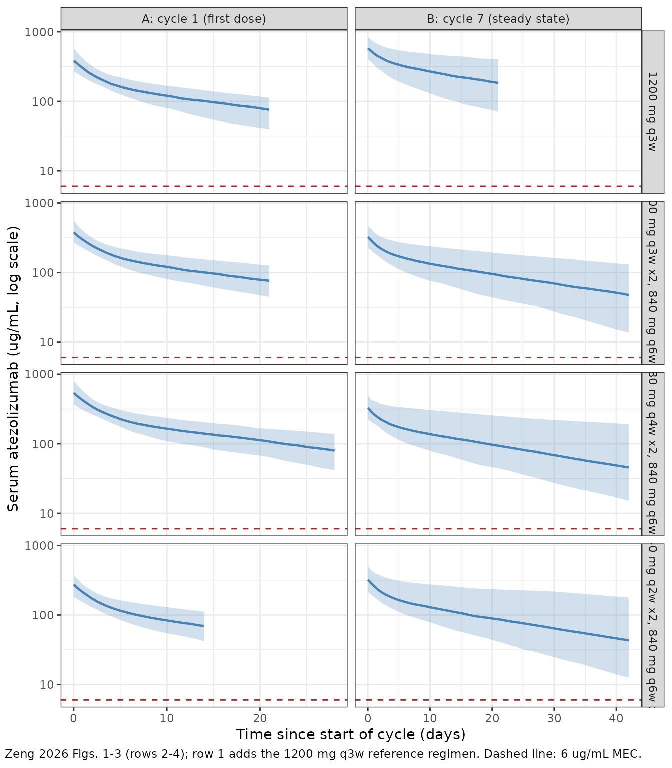
The paper’s substantive claim about every extended-interval regimen is that the trough stays “well above the target concentration”. Checked on the 5th percentile of the cycle-7 profile:
mec_tbl <- ribbon |>
  filter(cycle == 7L) |>
  group_by(regimen) |>
  summarise(`5th pctile trough` = min(lo), `median trough` = min(md),
            .groups = "drop")
knitr::kable(mec_tbl, digits = 1, caption = "Cycle 7 minima; MEC is 6 ug/mL.")| regimen | 5th pctile trough | median trough |
|---|---|---|
| 1200 mg q3w | 70.4 | 182.6 |
| 1200 mg q3w x2, 840 mg q6w x5 | 14.6 | 47.0 |
| 1680 mg q4w x2, 840 mg q6w x5 | 12.3 | 48.7 |
| 840 mg q2w x2, 840 mg q6w x5 | 12.6 | 43.9 |
PKNCA validation and comparison against the published exposures
Zeng 2026 Table 2 reports geometric means (90% PI) over 1000 virtual patients for each regimen and cycle, in each of the three softwares. The RxODE column is the apples-to-apples reference for an rxode2 reimplementation, so it is the one compared here.
nca_all <- nca_by_arm(sim_all)
#> No dose information provided, calculations requiring dose will return NA.
nca_gm <- geo_summary(nca_all)
# Every arm must yield every metric. A missing Ctrough renders as a blank cell
# in the comparison table below, which reads as agreement rather than as a gap.
stopifnot(
  nrow(nca_all) == 200 * 8 * 4,
  !any(is.na(nca_all$PPORRES)),
  nrow(nca_gm) == 8 * 4,
  !any(is.na(nca_gm$PPORRES))
)
ref_table2 <- tibble::tribble(
  ~regimen,                        ~cycle, ~cmax, ~ctrough, ~auclast,
  "1200 mg q3w",                       1L,   386,     71.6,      967,
  "1200 mg q3w",                       7L,   577,    187.0,     2043,
  "840 mg q2w x2, 840 mg q6w x5",      1L,   270,     67.7,      808,
  "840 mg q2w x2, 840 mg q6w x5",      7L,   328,     47.5,      771,
  "1200 mg q3w x2, 840 mg q6w x5",     1L,   386,     71.6,      967,
  "1200 mg q3w x2, 840 mg q6w x5",     7L,   329,     47.7,      774,
  "1680 mg q4w x2, 840 mg q6w x5",     1L,   540,     74.9,     1171,
  "1680 mg q4w x2, 840 mg q6w x5",     7L,   330,     48.0,      745
) |>
  mutate(arm = paste(regimen, "cycle", cycle)) |>
  select(arm, cmax, ctrough, auclast) |>
  as.data.frame()

tbl_pub <- nlmixr2lib::ncaComparisonTable(
  nca_gm |> filter(PPTESTCD != "tmax") |> as.data.frame(),
  ref_table2, by = "arm",
  units = c(cmax = "ug/mL", ctrough = "ug/mL", auclast = "ug*day/mL"),
  tolerance_pct = 15
)
knitr::kable(tbl_pub, digits = 1, row.names = FALSE,
caption = "Simulated (n = 200, IIV on) vs Zeng 2026 Table 2 RxODE column (n = 1000). auclast rows are weekly AUC.")| NCA parameter | arm | Reference | Simulated | % diff |
|---|---|---|---|---|
| Cmax (ug/mL) | 1200 mg q3w cycle 1 | 386 | 390 | +1.0% |
| Cmax (ug/mL) | 1200 mg q3w cycle 7 | 577 | 578 | +0.1% |
| Cmax (ug/mL) | 840 mg q2w x2, 840 mg q6w x5 cycle 1 | 270 | 266 | -1.5% |
| Cmax (ug/mL) | 840 mg q2w x2, 840 mg q6w x5 cycle 7 | 328 | 322 | -2.0% |
| Cmax (ug/mL) | 1200 mg q3w x2, 840 mg q6w x5 cycle 1 | 386 | 377 | -2.3% |
| Cmax (ug/mL) | 1200 mg q3w x2, 840 mg q6w x5 cycle 7 | 329 | 319 | -3.0% |
| Cmax (ug/mL) | 1680 mg q4w x2, 840 mg q6w x5 cycle 1 | 540 | 540 | -0.1% |
| Cmax (ug/mL) | 1680 mg q4w x2, 840 mg q6w x5 cycle 7 | 330 | 328 | -0.7% |
| AUClast (ug*day/mL) | 1200 mg q3w cycle 1 | 967 | 972 | +0.5% |
| AUClast (ug*day/mL) | 1200 mg q3w cycle 7 | 2040 | 1980 | -3.0% |
| AUClast (ug*day/mL) | 840 mg q2w x2, 840 mg q6w x5 cycle 1 | 808 | 806 | -0.3% |
| AUClast (ug*day/mL) | 840 mg q2w x2, 840 mg q6w x5 cycle 7 | 771 | 738 | -4.3% |
| AUClast (ug*day/mL) | 1200 mg q3w x2, 840 mg q6w x5 cycle 1 | 967 | 972 | +0.5% |
| AUClast (ug*day/mL) | 1200 mg q3w x2, 840 mg q6w x5 cycle 7 | 774 | 755 | -2.5% |
| AUClast (ug*day/mL) | 1680 mg q4w x2, 840 mg q6w x5 cycle 1 | 1170 | 1160 | -0.6% |
| AUClast (ug*day/mL) | 1680 mg q4w x2, 840 mg q6w x5 cycle 7 | 745 | 749 | +0.5% |
| Ctrough (ug/mL) | 1200 mg q3w cycle 1 | 71.6 | 71.4 | -0.3% |
| Ctrough (ug/mL) | 1200 mg q3w cycle 7 | 187 | 176 | -5.7% |
| Ctrough (ug/mL) | 840 mg q2w x2, 840 mg q6w x5 cycle 1 | 67.7 | 67.7 | -0.0% |
| Ctrough (ug/mL) | 840 mg q2w x2, 840 mg q6w x5 cycle 7 | 47.5 | 43.1 | -9.2% |
| Ctrough (ug/mL) | 1200 mg q3w x2, 840 mg q6w x5 cycle 1 | 71.6 | 73.1 | +2.1% |
| Ctrough (ug/mL) | 1200 mg q3w x2, 840 mg q6w x5 cycle 7 | 47.7 | 46.2 | -3.2% |
| Ctrough (ug/mL) | 1680 mg q4w x2, 840 mg q6w x5 cycle 1 | 74.9 | 75.1 | +0.3% |
| Ctrough (ug/mL) | 1680 mg q4w x2, 840 mg q6w x5 cycle 7 | 48 | 44.8 | -6.6% |
A built-in noise ruler
The scatter above needs a scale, and this design supplies one without any extra assumption. Cycle 1 of the “1200 mg q3w” regimen and cycle 1 of the “1200 mg q3w x2 then 840 mg q6w” regimen are the same dosing history, so the paper reports identical Table 2 values for both. They were simulated here as two independent arms with independent random-effect draws, so the difference between the two simulated values is pure Monte Carlo noise with a known true difference of zero.
noise <- nca_gm |>
  filter(arm %in% c("1200 mg q3w cycle 1",
                    "1200 mg q3w x2, 840 mg q6w x5 cycle 1"),
         PPTESTCD != "tmax") |>
  tidyr::pivot_wider(names_from = arm, values_from = PPORRES) |>
  mutate(`noise (%)` = 100 *
           (`1200 mg q3w x2, 840 mg q6w x5 cycle 1` - `1200 mg q3w cycle 1`) /
           `1200 mg q3w cycle 1`)
knitr::kable(noise, digits = 2,
caption = "Two identical designs simulated independently; the true difference is zero.")| PPTESTCD | 1200 mg q3w cycle 1 | 1200 mg q3w x2, 840 mg q6w x5 cycle 1 | noise (%) |
|---|---|---|---|
| auclast | 971.90 | 971.66 | -0.02 |
| cmax | 389.92 | 377.22 | -3.26 |
| ctrough | 71.39 | 73.08 | 2.37 |
Every Cmax and Ctrough deviation in the comparison table is of this order or smaller, so those residual differences are consistent with sampling noise rather than with a structural discrepancy.
A second ruler covers the weekly-AUC column, whose largest deviation (the 1680 mg q4w arm at cycle 7) exceeds the first ruler. All three extended-interval regimens have converged onto the same 840 mg q6w maintenance dosing by cycle 7, differing only in whether the seventh dose falls on day 224, 231 or 238, so their cycle-7 exposures should be nearly identical. The spread across those three rows within the published table is therefore a measure of the paper’s own simulation noise, and it is the same size as ours.
ss_arms <- paste(c("840 mg q2w x2, 840 mg q6w x5", "1200 mg q3w x2, 840 mg q6w x5",
                   "1680 mg q4w x2, 840 mg q6w x5"), "cycle 7")
spread <- function(x) 100 * (max(x) - min(x)) / min(x)
bind_rows(
  ref_table2 |> filter(arm %in% ss_arms) |>
    select(arm, cmax, ctrough, auclast) |>
    tidyr::pivot_longer(-arm, names_to = "PPTESTCD", values_to = "value") |>
    mutate(Source = "Zeng 2026 Table 2 (n = 1000)"),
  nca_gm |> filter(arm %in% ss_arms, PPTESTCD != "tmax") |>
    rename(value = PPORRES) |> mutate(Source = "Reproduced (n = 200)")
) |>
  group_by(Source, PPTESTCD) |>
  summarise(`spread across the 3 arms (%)` = spread(value), .groups = "drop") |>
  tidyr::pivot_wider(names_from = Source,
                     values_from = `spread across the 3 arms (%)`) |>
  knitr::kable(digits = 2,
caption = "Three arms that share the same steady-state maintenance dosing; the spread within each source is that source's own simulation noise.")| PPTESTCD | Reproduced (n = 200) | Zeng 2026 Table 2 (n = 1000) |
|---|---|---|
| auclast | 2.21 | 3.89 |
| cmax | 2.63 | 0.61 |
| ctrough | 7.12 | 1.05 |
Monte Carlo error is the dominant residual difference
The comparison above is a 200-subject cohort against a 1000-subject
one, with an independent IIV draw. cl_time_max carries an
IIV variance of 0.804609, so the cycle-7 trough is by far the most
dispersed metric and the least precisely estimated in either cohort. The
sampling noise below is the scale against which any remaining gap should
be read.
nca_all |>
  filter(PPTESTCD %in% c("cmax", "ctrough", "auclast")) |>
  group_by(arm, PPTESTCD) |>
  summarise(sd_log = sd(log(pmax(PPORRES, 1e-12))), n = dplyr::n(),
            .groups = "drop") |>
  group_by(PPTESTCD) |>
  summarise(
    `median between-subject CV (%)` = 100 * median(sd_log),
    `SE of geometric mean at n=200 (%)` = 100 * median(sd_log) / sqrt(200),
    `SE at the paper's n=1000 (%)` = 100 * median(sd_log) / sqrt(1000),
    .groups = "drop"
  ) |>
knitr::kable(digits = 2)| PPTESTCD | median between-subject CV (%) | SE of geometric mean at n=200 (%) | SE at the paper’s n=1000 (%) |
|---|---|---|---|
| auclast | 28.80 | 2.04 | 0.91 |
| cmax | 23.33 | 1.65 | 0.74 |
| ctrough | 46.97 | 3.32 | 1.49 |
Internal consistency of the published table
One structural check that needs no simulation at all: cycle 1 of the “1200 mg q3w x2 then 840 mg q6w” regimen is, by construction, identical to cycle 1 of the standard “1200 mg q3w” regimen. Table 2 reports identical values for both rows in all three softwares, which independently confirms the regimen encoding used here.
ref_table2 |>
  filter(arm %in% c("1200 mg q3w cycle 1",
                    "1200 mg q3w x2, 840 mg q6w x5 cycle 1")) |>
knitr::kable(row.names = FALSE)| arm | cmax | ctrough | auclast |
|---|---|---|---|
| 1200 mg q3w cycle 1 | 386 | 71.6 | 967 |
| 1200 mg q3w x2, 840 mg q6w x5 cycle 1 | 386 | 71.6 | 967 |
Assumptions and deviations
- The parameter values are not this paper’s own estimates. They are transcribed by the authors from the FDA CDER clinical pharmacology and biopharmaceutics review for BLA 761041Orig1s000, which was not available when this model was built. Zeng 2026 is the transcription source and the only source consulted here. If the FDA review is obtained later, the values, the covariate reference points and the omega scale should be re-checked against it. The same model underpins Peer et al. J Clin Pharmacol 2023;63(6):672-680, also not available when this model was built.
-
Everything is
fixed(). No parameter in this model was estimated from data in this paper. All 17$THETA, all 4$OMEGAand$SIGMAcarryFIXin the source control stream. -
Residual error follows the NONMEM
$ERRORblock, i.e. combined proportional (SD 0.034) plus additive (SD 18.1 ug/mL). The supplement’s three implementations do not agree here. The Pumas@derivedblock usesNormal(cp, sigma_add + sqrt(cp^2 * sigma2_prop)), which adds the two standard deviations and treats 0.034 as a variance (an 18.4% proportional SD); the RxODE snippet writescp = C1 + sqrt(C1^2 * prop^2 + add^2), which adds a standard deviation to the prediction deterministically instead of sampling. The NONMEM stream is the direct transcription of the FDA review and itsW = sqrt(prop^2 * IPRED^2 + add^2)is the standard combined form, so it is the one encoded. This affects only residual error, not the exposures validated above, which are model predictions. -
The
$THETAcomment labels contradict the$ERRORequation. The stream annotatesTHETA(1)as “exponential error” andTHETA(2)as “additive error”, but$ERRORuses both as standard deviations in a combined additive-plus-proportional variance function. The equation governs. -
Infusion duration is unstated.
$INPUTdeclares aRATEcolumn but no duration or rate value appears anywhere in the paper or supplement. Doses are simulated as boluses; the Infusion duration section quantifies the effect on Cmax as about 1% for a 60-minute infusion (258.4 vs 255.9 ug/mL). -
Two unit typos in the source Methods text, resolved against
Table 1 and the generating code. Albumin is described as “a
mean of 42 g/dL” but is g/L (Table 1 header, median 42.0-42.2, and the
covariate reference of 40); baseline tumor burden is described as “a
mean of 4.2 mm^3” but 4.2 is the
meanlogof a lognormal in mm (Table 1 header, median 67.5-69.3 mm). - The loading interval of the third extended-interval regimen is q4w. The Methods sentence says “1680 mg Q6W”, but Table 2, Table 3 and the Fig. 3 caption say q4w, and the Results text describes Fig. 3 as “1680 mg Q4W followed by 840 mg Q6W”. Table 3 separately mislabels the second regimen as “1200 mg q4w” where Table 2 has q3w. The Table 2 and figure-caption labels are used.
- Supplemental Table 1’s summary statistic is unstated, and its parenthetical intervals are narrower than the 90% prediction intervals of the reproduced cohort. Only its central values are used as targets; see the trough discussion above.
-
Age is not a model covariate. It appears in
$INPUTand in the population-generation code, where it drives body weight, but no$PKterm uses it. It is recorded incovariatesDataExcludedrather thancovariateData. - Cohort size. 200 per arm here versus 1000 in the paper, per the nlmixr2lib cohort cap; both are prefixes of the paper’s own n = 1000 draw. The deterministic arm uses the first 100, which is what Supplemental Table 1 used.
- The comparison targets are simulated, not observed. No observed atezolizumab concentrations appear in this paper, so no predictive check against clinical data is possible from this source. What the validation here establishes is that the nlmixr2lib encoding reproduces the published model, which is the strongest claim the source supports.