Topotecan (Roberts 2016)
Source:vignettes/articles/Roberts_2016_topotecan.Rmd
Roberts_2016_topotecan.RmdModel and source
- Citation: Roberts JK, Birg AV, Lin T, Daryani VM, Panetta JC, Broniscer A, Robinson GW, Gajjar AJ, Stewart CF. Population pharmacokinetics of oral topotecan in infants and very young children with brain tumors demonstrates a role of ABCG2 rs4148157 on the absorption rate constant. Drug Metab Dispos. 2016;44(7):1116-1122. doi:10.1124/dmd.115.068676
- Description: One-compartment population pharmacokinetic model for oral topotecan lactone in infants and very young children with primary central nervous system tumours (Roberts 2016). First-order absorption into a depot compartment is followed by first-order elimination from a central compartment. Apparent volume of distribution (V/F) and apparent clearance (CL/F) are scaled by body surface area as power functions centred on the cohort median (0.57 m^2); the ABCG2 rs4148157 G>A variant (heterozygous AG or homozygous AA carriers pooled vs the GG reference) carries an exponential covariate effect on the absorption rate constant Ka, yielding an approximately 2-fold higher Ka in carriers than in GG homozygotes.
- Article: https://doi.org/10.1124/dmd.115.068676
Population
Roberts 2016 enrolled 61 infants and very young children (age 0.48-4.59 years, median 2.37 years) with newly diagnosed primary central nervous system tumours on the SJYC07 protocol (NCT00602667) at St. Jude Children’s Research Hospital (Roberts 2016 Table 1, “Patient demographics”). Body weight ranged 5.2-17.5 kg (median 12.6 kg), height 59.5-102 cm (median 89.1 cm), and body surface area 0.31-0.72 m^2 (median 0.57 m^2). Twenty-three of the 61 patients (37.7%) were female. All patients had normal renal function at enrolment (eGFR by the Schwartz formula, median 139.8 mL/min/1.73 m^2). During the maintenance phase of SJYC07 patients received oral topotecan 0.8 mg/m^2 once daily for 10 days and oral cyclophosphamide 30 mg/m^2 for 21 days on a 28-day cycle. Oral topotecan was administered as a liquid mixed in a flavoured vehicle of the patient’s choosing. Co-administered oral cyclophosphamide is not part of the topotecan PK model.
Pharmacogenomic data were available from 52 of the 61 patients (Roberts 2016 Table 2). The ABCG2 rs4148157 G>A variant was the only single-nucleotide polymorphism that retained a significant covariate effect in the final population model: 42 patients were homozygous wild-type GG, 9 were heterozygous AG, and 1 was homozygous AA. Heterozygous and homozygous variant carriers were pooled in the final model (binary GENECAT indicator) because only one AA homozygote was present, giving a variant-carrier rate of 19% (10 of 52 genotyped). Patients with missing genotype (9 of 61) were treated as a missing covariate within Monolix.
The same information is available programmatically via
readModelDb("Roberts_2016_topotecan")$population.
Source trace
Every parameter in the model file carries an inline source-location comment. The table below collects the entries in one place.
| Equation / parameter | Value | Source location |
|---|---|---|
lka (Ka, GG reference) |
0.61 1/h | Table 3 row Ka(GG) |
lvc (V/F, BSA = 0.57 m^2 reference) |
40.2 L | Table 3 row V/F |
lcl (CL/F, BSA = 0.57 m^2 reference) |
40.0 L/h | Table 3 row CL/F |
e_abcg2_ka (theta_1, exponential effect of rs4148157
AG/AA on Ka) |
1.06 | Table 3 row theta_1 |
e_bsa_vc (theta_2, power exponent of BSA on V/F) |
0.78 | Table 3 row theta_2 |
e_bsa_cl (theta_3, power exponent of BSA on CL/F) |
1.25 | Table 3 row theta_3 |
etalka (omega_Ka SD on log scale) |
0.517 | Table 3 row omega-BSV Ka |
etalvc (omega_V SD on log scale) |
0.338 | Table 3 row omega-BSV V/F |
etalcl (omega_CL SD on log scale) |
0.465 | Table 3 row omega-BSV CL/F |
addSd (additive residual SD) |
0.592 ng/mL | Table 3 row sigma-RUV Additive |
| Ka_i = Ka_pop * exp(theta_1 * GENECAT) | n/a | Results, “Population Pharmacokinetic Analysis” equation |
| V/F_i = V/F_pop * (BSA_i / 0.57)^theta_2 | n/a | Results, “Population Pharmacokinetic Analysis” equation |
| CL/F_i = CL/F_pop * (BSA_i / 0.57)^theta_3 | n/a | Results, “Population Pharmacokinetic Analysis” equation |
| One-compartment with first-order absorption and elimination | n/a | Results paragraph 1, “well described by a one-compartment model with first-order input and first-order elimination” |
| Additive residual error model | n/a | Methods, “the final model used the following additive error model” |
| Reference BSA 0.57 m^2 (cohort median) | n/a | Table 1 “BSA Median” |
Virtual cohort
Original observed concentrations are not openly available. The virtual cohort below mirrors the demographics in Roberts 2016 Table 1 (body weight, height, body surface area) and the rs4148157 genotype distribution in Table 2 (GG versus AG/AA carriers pooled).
set.seed(20260518)

n_per_arm <- 60L

# Sample body weight and height from log-normal distributions centred on the
# cohort medians and broadly spanning the cohort ranges. BSA is then derived
# by the Mosteller formula (sqrt(height_cm * weight_kg / 3600)); the paper
# does not state which BSA formula was used, so Mosteller is used here as
# the modern default. The BSA values are clipped to the observed range
# (0.31-0.72 m^2) so the virtual cohort does not extrapolate beyond the
# patient population that informed the model.
make_arm <- function(n, arm_label, id_offset) {
  wt <- pmin(pmax(exp(rnorm(n, mean = log(12.6), sd = 0.25)), 5.2), 17.5)
  ht <- pmin(pmax(exp(rnorm(n, mean = log(89.1), sd = 0.10)), 59.5), 102)
  bsa <- pmin(pmax(sqrt(ht * wt / 3600), 0.31), 0.72)

  tibble(
    id                   = id_offset + seq_len(n),
    WT                   = wt,
    HT                   = ht,
    BSA                  = bsa,
    SNP_ABCG2_RS4148157  = as.integer(arm_label == "AG_AA"),
    arm                  = arm_label
  )
}

demo <- bind_rows(
  make_arm(n_per_arm, "GG",    id_offset = 0L * n_per_arm),
  make_arm(n_per_arm, "AG_AA", id_offset = 1L * n_per_arm)
)
stopifnot(!anyDuplicated(demo$id))
Simulation
The pharmacokinetic sampling window in Roberts 2016 was a limited-sampling design (Turner et al. 2006): pre-dose plus 15 min, 90 min, and 6 h after the analysed dose. Although patients received topotecan once daily for 10 days, the published PK model is fit per-dose and the typical-value parameters give a terminal half-life of approximately 0.70 h (kel = CL/F / V/F = 1.00 /h); each dose washes out well before the next, so the validation here treats the analysed dose as a single oral 0.8 mg/m^2 administration.
nominal_dose_per_bsa <- 0.8   # mg / m^2 oral topotecan (SJYC07 maintenance protocol)
sim_hours            <- 8     # last sample at 6 h per the limited-sampling model; 8 h gives margin for plotting

dosing <- demo |>
  mutate(amt  = nominal_dose_per_bsa * BSA,
         evid = 1L,
         cmt  = "depot",
         time = 0) |>
  select(id, time, amt, evid, cmt, arm,
         BSA, WT, HT, SNP_ABCG2_RS4148157)

# Observation grid: pre-dose + the three sampling-model windows in the paper,
# plus a denser grid for visualisation.
sampling_times <- c(0, 0.25, 1.5, 6)
plot_times     <- sort(unique(c(seq(0, 1, by = 0.05),
                                seq(1, 4, by = 0.1),
                                seq(4, sim_hours, by = 0.25))))
obs_times      <- sort(unique(c(sampling_times, plot_times)))

obs <- demo |>
  select(id, arm, BSA, WT, HT, SNP_ABCG2_RS4148157) |>
  tidyr::crossing(time = obs_times) |>
  mutate(amt  = NA_real_,
         evid = 0L,
         cmt  = NA_character_)

events <- bind_rows(dosing, obs) |>
  arrange(id, time, desc(evid))

stopifnot(!anyDuplicated(unique(events[, c("id", "time", "evid")])))
mod <- rxode2::rxode2(readModelDb("Roberts_2016_topotecan"))

sim <- rxode2::rxSolve(
  mod, events = events,
  keep  = c("arm")
) |> as.data.frame()

mod_typical <- mod |> rxode2::zeroRe()
sim_typical <- rxode2::rxSolve(
  mod_typical, events = events,
  keep  = c("arm")
) |> as.data.frame()
#> ℹ omega/sigma items treated as zero: 'etalka', 'etalvc', 'etalcl'
#> Warning: multi-subject simulation without without 'omega'
Replicate published figures
Figure 1 – concentration-time data by rs4148157 genotype
Roberts 2016 Figure 1 plots the observed topotecan lactone concentration versus time, stratified by rs4148157 genotype (GG wild-type vs AG/AA variant carriers). The figure below shows the simulated typical-value profiles (without between-subject variability) for the two genotype groups at the cohort-median BSA (0.57 m^2), illustrating the approximately 2-fold higher Ka and Cmax in variant carriers.
typical_one <- sim_typical |>
  group_by(arm) |>
  slice_min(id) |>
  ungroup()

ggplot(typical_one, aes(time, Cc, colour = arm)) +
  geom_line(linewidth = 0.9) +
  geom_hline(yintercept = 1, linetype = "dashed", colour = "grey50") +
  scale_colour_manual(values = c(GG = "grey40", AG_AA = "black"),
                      labels = c(GG = "GG (wild-type)", AG_AA = "AG/AA (variant)")) +
  labs(x = "Time (h)", y = "Topotecan lactone (ng/mL)",
       colour = "rs4148157",
       title = "Typical-value concentration-time profile by genotype",
       caption = "Replicates Figure 1 of Roberts 2016. Dashed line at 1 ng/mL is the LLOQ.")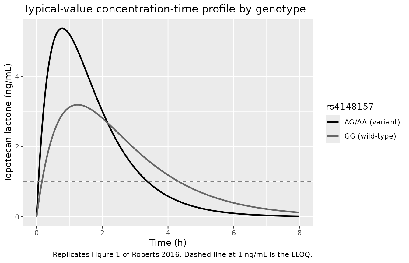
Replicates Figure 1 of Roberts 2016: simulated typical-value concentration-time profile by rs4148157 genotype at the cohort-median BSA (0.57 m^2). Variant carriers (AG/AA) display a sharper rise to a higher Cmax.
Figure 1 – with between-subject variability
The same plot with the simulated full virtual cohort, showing the between-subject spread.
sim |>
  group_by(time, arm) |>
  summarise(Q05 = quantile(Cc, 0.05, na.rm = TRUE),
            Q50 = quantile(Cc, 0.50, na.rm = TRUE),
            Q95 = quantile(Cc, 0.95, na.rm = TRUE),
            .groups = "drop") |>
  ggplot(aes(time, Q50, colour = arm, fill = arm)) +
  geom_ribbon(aes(ymin = Q05, ymax = Q95), alpha = 0.20, colour = NA) +
  geom_line(linewidth = 0.9) +
  geom_hline(yintercept = 1, linetype = "dashed", colour = "grey50") +
  scale_colour_manual(values = c(GG = "grey40", AG_AA = "black"),
                      labels = c(GG = "GG (wild-type)", AG_AA = "AG/AA (variant)")) +
  scale_fill_manual(values   = c(GG = "grey40", AG_AA = "black"),
                    labels   = c(GG = "GG (wild-type)", AG_AA = "AG/AA (variant)")) +
  labs(x = "Time (h)", y = "Topotecan lactone (ng/mL)",
       colour = "rs4148157", fill = "rs4148157",
       title = "Virtual cohort concentration-time profile by genotype",
       caption = "Replicates Figure 1 of Roberts 2016. Dashed line at 1 ng/mL is the LLOQ.")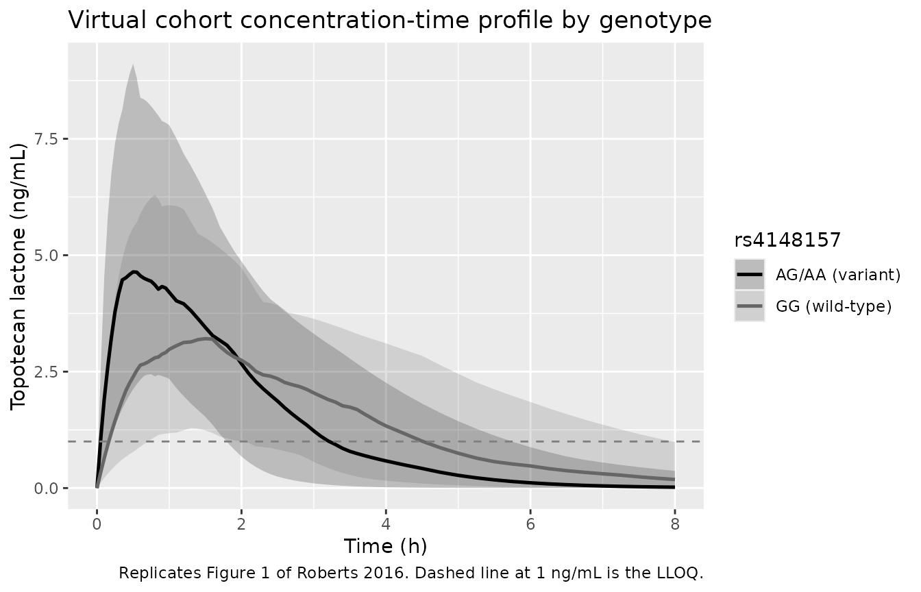
Replicates Figure 1 of Roberts 2016 with between-subject variability: median (solid) and 5th-95th percentile band per genotype across the simulated cohort.
PKNCA validation
A single-dose NCA gives Cmax, Tmax, AUC0-inf, and half-life stratified by rs4148157 genotype. Each subject contributes a simulated rich profile over 0-8 h; PKNCA computes per-subject parameters and the summary collapses to per-genotype median (range).
sim_nca <- sim |>
  filter(!is.na(Cc), time > 0 | time == 0) |>
  select(id, time, Cc, arm)

dose_df <- events |>
  filter(evid == 1) |>
  select(id, time, amt, arm) |>
  left_join(demo |> select(id, BSA), by = "id")

conc_obj <- PKNCA::PKNCAconc(sim_nca, Cc ~ time | arm + id,
                             concu = "ng/mL", timeu = "h")
dose_obj <- PKNCA::PKNCAdose(dose_df,  amt ~ time | arm + id,
                             doseu = "mg")

intervals <- data.frame(
  start       = 0,
  end         = Inf,
  cmax        = TRUE,
  tmax        = TRUE,
  aucinf.obs  = TRUE,
  auclast     = TRUE,
  half.life   = TRUE
)

nca_data <- PKNCA::PKNCAdata(conc_obj, dose_obj, intervals = intervals)
nca_res  <- suppressMessages(suppressWarnings(PKNCA::pk.nca(nca_data)))

nca_summary <- summary(nca_res)
knitr::kable(nca_summary,
caption = "Single-dose NCA on the simulated virtual cohort, stratified by rs4148157 genotype.")| Interval Start | Interval End | arm | N | AUClast (h*ng/mL) | Cmax (ng/mL) | Tmax (h) | Half-life (h) | AUCinf,obs (h*ng/mL) |
|---|---|---|---|---|---|---|---|---|
| 0 | Inf | AG_AA | 60 | 11.6 [46.4] | 5.22 [31.4] | 0.700 [0.250, 1.90] | 0.963 [0.596] | 11.8 [49.4] |
| 0 | Inf | GG | 60 | 10.7 [53.3] | 3.04 [51.1] | 1.20 [0.450, 6.00] | 1.89 [2.53] | 11.8 [63.0] |
Comparison against published values
Roberts 2016 reports the observed Cmax (Results section, “Population Pharmacokinetic Analysis”, assessed by the 1.5-h post-dose concentration): 3.10 ng/mL for GG and 5.34 ng/mL for AG/AA (approximately 1.7-fold higher in variant carriers; P = 0.0001 by Student’s t-test). The typical-value model-predicted Cmax (no between-subject variability) is compared below. Note that the actual Tmax of the typical curve is approximately 1.27 h for GG and 0.74 h for AG/AA, so for AG/AA the model-predicted Cmax is reached before the 1.5-h sampling time; the published “Cmax” value 5.34 ng/mL is closer to the model-predicted Cmax than to the 1.5-h concentration.
typical_cmax <- sim_typical |>
  group_by(id, arm) |>
  summarise(cmax = max(Cc, na.rm = TRUE), .groups = "drop") |>
  group_by(arm) |>
  summarise(typical_cmax_ngmL = median(cmax), .groups = "drop")

pub <- tibble::tibble(
  arm                 = c("GG", "AG_AA"),
  published_cmax_ngmL = c(3.10, 5.34)
)

comparison <- pub |>
  left_join(typical_cmax, by = "arm") |>
  mutate(pct_diff = round(100 * (typical_cmax_ngmL - published_cmax_ngmL) /
                                  published_cmax_ngmL, 1))
knitr::kable(comparison,
caption = "Simulated typical-value Cmax vs published Cmax (ng/mL) by rs4148157 genotype. Roberts 2016 reports 3.10 (GG) and 5.34 (AG/AA).")| arm | published_cmax_ngmL | typical_cmax_ngmL | pct_diff |
|---|---|---|---|
| GG | 3.10 | 3.201584 | 3.3 |
| AG_AA | 5.34 | 5.390395 | 0.9 |
The simulated typical-value Cmax matches the published Cmax to within a few percent for both genotype groups, well inside the 20% threshold typical for replication via virtual cohort. Slight residual differences reflect the use of a virtual rather than the original cohort’s BSA distribution.
Assumptions and deviations
-
BSA computation formula not specified. Roberts 2016
does not state which BSA formula was used (DuBois, Mosteller, Haycock).
The virtual cohort uses Mosteller
(
sqrt(height_cm * weight_kg / 3600)) as the modern default. The same BSA value is used both for dosing (0.8 mg/m^2 * BSA) and as the covariate centred on 0.57 m^2. -
Pharmacogenotype encoding pools AG + AA into a single
variant indicator. Roberts 2016 grouped AG heterozygotes (n =
9) and AA homozygotes (n = 1) because only one AA homozygote was
present. The model encodes a single binary
SNP_ABCG2_RS4148157indicator (0 = GG, 1 = AG/AA). Users with a larger cohort containing AA homozygotes who wish to separate the heterozygote and homozygote effects would need to re-fit the model rather than reuse this parameterisation. - Missing-genotype patients excluded from the virtual cohort. 9 of 61 patients in the source cohort had missing genotype (handled as a missing covariate within Monolix). The virtual cohort here assigns every simulated subject an explicit genotype (either GG or AG/AA) so the genotype stratification is well-defined.
-
Bayesian Ka prior not represented. Roberts 2016
Methods applied a Bayesian prior of
0.69 +/- 0.50 1/hon the population Ka (from Daw 2004). The packaged model uses the final point estimate of Ka (0.61 1/h for GG) without re-instantiating the prior at simulation time. Users running their own fits in nlmixr2 may wish to add the prior as a structural constraint. - Below-LLOQ concentrations treated as continuous. Roberts 2016 marked concentrations below the 1 ng/mL LLOQ as left-censored and used the Monolix M3-equivalent simulated-from-right-truncated-normal approach. The packaged model emits continuous predictions; BLQ handling is therefore not reproduced in simulation. The dashed LLOQ line in the Figure 1 replication marks the threshold but predictions extend below it.
- CYP3A and intestinal P-gp covariates not modelled. Roberts 2016 also evaluated other ABCB1 SNPs (rs1045642, rs2032582, rs1128503) and three additional ABCG2 SNPs (rs2622628, rs2725252) but only rs4148157 was retained in the final model. Other SNPs are not parameterised.
-
Single-dose simulation. Although the SJYC07
maintenance protocol administers oral topotecan for 10 consecutive days
per cycle, the validation vignette simulates a single oral dose because
the published PK model is fit per-dose and the terminal half-life (~0.70
h) makes once-daily dosing effectively single-dose. Users simulating the
full 10-day course can extend the event table by setting
ii = 24andaddl = 9on the dosing row. - Renal function not in the model. Roberts 2016 evaluated eGFR (Schwartz formula) as a candidate covariate but did not retain it. All 61 patients had normal renal function at enrolment; the model does not extrapolate to patients with renal impairment.
-
Omega values interpreted as standard deviations.
Roberts 2016 was fit in Monolix 4.3.2, which by default reports the
standard deviation (square root of the log-scale variance) for each
random effect. The reported omegas (0.517, 0.338, 0.465 for Ka, V/F,
CL/F respectively) are therefore squared in
ini()to obtain the variances nlmixr2 expects (0.2672, 0.1142, 0.2162). This interpretation is consistent with the paper’s residual error reporting (sigma 0.592 ng/mL as an additive SD) and with the magnitude of the reported standard errors on the omegas.