Mitoxantrone (Brandon 2026)
Source:vignettes/articles/Brandon_2026_mitoxantrone.Rmd
Brandon_2026_mitoxantrone.RmdModel and source
#> ℹ parameter labels from comments will be replaced by 'label()'Citation: Brandon AM, Huisman-Siebinga H, Barnett S, Wetherell P, Kearns P, Gibson B, Heaney N, Smith O, Baruchel A, Petit A, Moore A, Ogungbenro K, Huitema ADR, Veal GJ. Population pharmacokinetics and dose-response relationships of mitoxantrone in children with acute myeloid leukaemia. Br J Clin Pharmacol. 2026;92(6):1760-1770. doi:10.1002/bcp.70436
Description: Two-compartment intravenous population PK model for mitoxantrone in children with acute myeloid leukaemia (Brandon 2026), developed from 282 plasma concentrations (45.7% below the 5 ng/mL assay LLOQ, handled by the likelihood-based M3 method) in 44 patients aged 0.9-17 years receiving 1-h infusions of 12 mg/m2/day, or 0.4 mg/kg/day for infants below 12 months, at or under 10 kg, or below 0.5 m2 body surface area. CL and Q carry a body-weight allometric exponent of 0.75 and Vc and Vp an exponent of 1, both referenced to the cohort median weight of 27.5 kg. Vc is fixed to the paediatric literature value of 23.2 L from O’Brien 2010 to stabilise the fit; interindividual variability is a correlated block on CL and Vp. No other covariate was retained in the final model.
Article: https://doi.org/10.1002/bcp.70436
Supplement (Supporting Information S1-S4, including the final NONMEM control stream): https://doi.org/10.1002/bcp.70436, Supporting Information file
BCP-92-1760-s001.docx
Mitoxantrone is an anthracenedione used in induction chemotherapy for paediatric acute myeloid leukaemia (AML). Brandon 2026 is the first dedicated paediatric population PK analysis of the drug, and it was motivated by a specific clinical question: infants below a protocol-defined age, weight or body-surface-area cut-off receive a reduced body-weight-based dose (0.4 mg/kg/day) instead of the standard 12 mg/m^2/day, and that reduction has never been justified pharmacokinetically. The model is therefore used in the paper mainly as an exposure calculator, and this vignette validates it the same way.
Population
The model was fit to 282 plasma mitoxantrone concentrations collected from 145 dosing events in 44 children enrolled in a single phase III AML trial (ISRCTN12389567; EudraCT 2014-005066-30) conducted in the UK, Ireland, France and Australia. Patients were aged 0.9-17.0 years (median 9.7) and weighed 9.5-69.5 kg (median 27.5); 17 of 44 (38.6%) were female. Forty had newly diagnosed AML, three had isolated myeloid sarcoma and one had high-risk myelodysplastic syndrome (Brandon 2026 Table 1).
Forty-one patients received the standard 12 mg/m^2/day 1-h intravenous infusion and three infants – aged 10-16 months and weighing 9.5-9.9 kg, all close to the eligibility cut-off – received the reduced 0.4 mg/kg/day regimen. The assay was HPLC with photo-diode-array detection (LLOQ 5 ng/mL); 45.7% of the modelled observations were below that limit, which is why the analysis used the likelihood-based M3 method rather than imputation or exclusion.
The same information is available programmatically via
readModelDb("Brandon_2026_mitoxantrone")()$population.
| Field | Value |
|---|---|
| species | human |
| n_subjects | 44 |
| n_studies | 1 |
| age_range | 0.9-17.0 years |
| age_median | 9.7 years |
| weight_range | 9.5-69.5 kg |
| weight_median | 27.5 kg |
| sex_female_pct | 38.6 |
| race_ethnicity | Not reported |
| disease_state | Newly diagnosed acute myeloid leukaemia (40 patients, 90.9%), isolated myeloid sarcoma (3, 6.8%) and high-risk myelodysplastic syndrome (1, 2.3%); all under 18 years at trial entry |
| dose_range | Mitoxantrone 12 mg/m2/day by 1-h intravenous infusion, once daily for up to 4 days. Infants below 12 months old, weighing 10 kg or less, or with a body surface area below 0.5 m2 instead received 0.4 mg/kg/day (3 of 44 patients). Administered dose 3.6-23 mg (median 12 mg); infusion duration 0.5-2.5 h (median 1.08 h). |
| regions | United Kingdom, Ireland, France and Australia |
| n_observations | 282 plasma concentrations from 145 dosing events, 45.7% below the 5 ng/mL LLOQ (313 samples were originally collected; artificially high end-of-infusion samples were excluded) |
| samples_plasma | Pre-dose; immediately after end of infusion on day 1; 0.5, 1, 2 and 6 h post-infusion on day 1; immediately before the day 2 infusion; and 48 and 72 h after the end of the final day’s infusion. Mean 7.1 samples per patient (range 3-8). |
| co_medication | All patients received non-chemotherapeutic concomitant medications for symptom and side-effect management; 16 of 44 (36.4%) received concomitant cytarabine (30-180 mg IV) within 7 days of starting mitoxantrone. |
| notes | Demographics from Brandon 2026 Table 1. Data came from a single phase III paediatric AML trial (ISRCTN12389567; EudraCT 2014-005066-30). Assay was HPLC with photo-diode-array detection, calibration range 5-1000 ng/mL and LLOQ 5 ng/mL. Estimation was by SAEM with a separate importance-sampling evaluation step, using the likelihood-based M3 method for the below-LLOQ observations. Serum creatinine, ALT and serum albumin were missing for two patients each and imputed as the population medians 36.0 umol/L, 42.5 U/L and 35.5 g/L. |
Source trace
Every ini() entry carries an in-file comment naming its
source location in
inst/modeldb/specificDrugs/Brandon_2026_mitoxantrone.R.
They are collected here for review. Table 2 of the paper and the
$THETA / $OMEGA records of the final NONMEM
control stream in Supporting Information S2 agree on every value, which
is what confirms these are final estimates rather than initial
values.
| Equation / parameter | Value | Source location |
|---|---|---|
lcl (CL at 27.5 kg) |
39.1 L/h (RSE 9.61%) | Table 2; supplement S2 $THETA (1) |
lvc (Vc, fixed) |
23.2 L | Table 2 “V1 23.2 fixed”; supplement S2 $THETA (2)
23.2 FIX; value from O’Brien 2010 (Results 3.2,
Discussion) |
lq (Q at 27.5 kg) |
27.6 L/h (RSE 25.0%) | Table 2; supplement S2 $THETA (3) |
lvp (Vp at 27.5 kg) |
85.9 L (RSE 22.6%) | Table 2; supplement S2 $THETA (4) |
e_wt_cl_q |
0.75 fixed | Table 2 “WT effect on CL, Q”; supplement S2 $THETA (5)
0.75 FIX
|
e_wt_vc_vp |
1 fixed | Table 2 “WT effect on V1, V2”; supplement S2 $THETA (6)
1 FIX
|
etalcl variance |
0.344 (64.0% CV, shrinkage 10.65%) | Supplement S2 $OMEGA BLOCK(2); Table 2 |
etalcl-etalvp covariance |
-0.426 (RSE 43.0%) | Supplement S2 $OMEGA BLOCK(2); Table 2 |
etalvp variance |
1.02 (133% CV, shrinkage 34.11%) | Supplement S2 $OMEGA BLOCK(2); Table 2 |
propSd |
0.382 (RSE 8.91%) | Table 2; supplement S2 $THETA (7) |
addSd |
2.5 ng/mL fixed | Table 2; supplement S2 $THETA (8) 2.5 FIX,
“1/2 LOQ” |
Allometric scaling TVP = theta * (WT/27.5)^k
|
n/a | Equation 1; supplement S2 $PK block |
Exponential IIV P_i = TVP * exp(eta_i)
|
n/a | Equation 2; supplement S2 $PK
CL = EXP(MU_1 + ETA(1))
|
| Two-compartment IV disposition | n/a | Results 3.2; supplement S2
$SUBROUTINES ADVAN3 TRANS4
|
Cc = central / vc * 1000 (mg/L to ng/mL) |
n/a | Supplement S2 $PK S1 = V1/1000
|
W = sqrt((prop * IPRED)^2 + add^2) |
n/a | Supplement S2 $ERROR block |
Omega scale
Table 2 reports the interindividual variability as CV% while the
estimated quantities are variances (Table 2 footnote: “IIV RSEs are
based on the standard errors of the estimated variances”). The two are
reconciled by the control stream, which prints the variances directly,
and the exact log-normal relation omega^2 = log(CV^2 + 1)
is what maps between them.
cv_printed <- c(CL = 0.640, Vp = 1.33)                # Table 2, CV% column
omega2_stream <- c(CL = 0.344, Vp = 1.02)             # Supplement S2 $OMEGA BLOCK(2)

omega2_exact  <- log(cv_printed^2 + 1)                # exact log-normal relation
omega2_approx <- cv_printed^2                         # the CV% = 100*sqrt(omega^2) shorthand

data.frame(
  Parameter              = names(cv_printed),
  `Printed CV`           = cv_printed,
  `Control stream omega2` = omega2_stream,
  `log(CV^2 + 1)`        = round(omega2_exact, 4),
  `CV^2`                 = round(omega2_approx, 4),
  check.names = FALSE, row.names = NULL
) |>
knitr::kable(caption = "The exact log-normal relation reproduces the control stream's variances; the CV^2 shorthand does not.")| Parameter | Printed CV | Control stream omega2 | log(CV^2 + 1) | CV^2 |
|---|---|---|---|---|
| CL | 0.64 | 0.344 | 0.3433 | 0.4096 |
| Vp | 1.33 | 1.020 | 1.0185 | 1.7689 |
# The exact relation agrees with the control stream to the precision the
# variances are printed to; the shorthand is off by 19% and 73%.
stopifnot(
  max(abs(omega2_exact - omega2_stream) / omega2_stream) < 0.01,
  min(abs(omega2_approx - omega2_stream) / omega2_stream) > 0.15
)

# The block must be positive definite for rxode2's Cholesky sampler.
omega_block <- matrix(c(0.344, -0.426, -0.426, 1.02), nrow = 2)
stopifnot(all(eigen(omega_block, only.values = TRUE)$values > 0))
cat("Implied CL-Vp correlation:",
    round(-0.426 / sqrt(0.344 * 1.02), 3), "\n")
#> Implied CL-Vp correlation: -0.719
Structural verification
These checks are deterministic: they use
rxode2::zeroRe() so there is no random draw, and each
compares the compiled ODE solution against a closed form that follows
from the published parameterisation. Tight bounds are therefore correct
here – the only source of disagreement is numerical integration
error.
mod     <- readModelDb("Brandon_2026_mitoxantrone")
mod_typ <- rxode2::zeroRe(mod)
#> ℹ parameter labels from comments will be replaced by 'label()'

# Reference values (Brandon 2026 Table 2), at the reference weight of 27.5 kg.
ref_wt <- 27.5
ref    <- c(cl = 39.1, vc = 23.2, q = 27.6, vp = 85.9)

# Observation grid: dense through the infusion and distribution phase, coarser
# through the terminal phase. Doses are single 1-h intravenous infusions, as in
# the simulations underlying Brandon 2026 Figure 4.
obs_times <- sort(unique(c(
  seq(0,  4,  by = 0.05),
  seq(4,  12, by = 0.25),
  seq(12, 72, by = 1)
)))

# Build an event table for one subject: a 1-h infusion into `central` (the ODE
# state, never the algebraic observable `Cc`) plus observations on that state.
make_subject <- function(id, wt, amt, infusion_h = 1) {
  dplyr::bind_rows(
    data.frame(id = id, time = 0, amt = amt, rate = amt / infusion_h,
               evid = 1L, cmt = "central"),
    data.frame(id = id, time = obs_times, amt = NA_real_, rate = NA_real_,
               evid = 0L, cmt = "central")
  ) |>
    dplyr::mutate(WT = wt)
}
Typical parameter values reproduce Table 2
ev_ref <- make_subject(1L, ref_wt, amt = 12)
s_ref  <- rxode2::rxSolve(mod_typ, ev_ref, atol = 1e-12, rtol = 1e-10,
                          returnType = "data.frame")
#> ℹ omega/sigma items treated as zero: 'etalcl', 'etalvp'

got <- c(cl = unique(s_ref$cl), vc = unique(s_ref$vc),
         q  = unique(s_ref$q),  vp = unique(s_ref$vp))

data.frame(Parameter = names(ref), `Table 2` = ref, Model = got,
           check.names = FALSE, row.names = NULL) |>
knitr::kable(caption = "Typical values at the reference body weight of 27.5 kg.")| Parameter | Table 2 | Model |
|---|---|---|
| cl | 39.1 | 39.1 |
| vc | 23.2 | 23.2 |
| q | 27.6 | 27.6 |
| vp | 85.9 | 85.9 |
Terminal half-life matches the analytic two-compartment root
# Analytic beta (slower) root of lambda^2 - (kel + k12 + k21) lambda + kel*k21.
beta_analytic <- function(cl, vc, q, vp) {
  kel <- cl / vc; k12 <- q / vc; k21 <- q / vp
  b <- kel + k12 + k21
  (b - sqrt(b^2 - 4 * kel * k21)) / 2
}

hl_analytic <- log(2) / beta_analytic(ref[["cl"]], ref[["vc"]], ref[["q"]], ref[["vp"]])

# Keep Cc >= 1e-6 * Cmax: below that the ODE integrator has no relative accuracy left.
tail_fit <- s_ref |> dplyr::filter(time >= 24, time <= 72, Cc >= 1e-6 * max(Cc, na.rm = TRUE))
hl_solve <- -log(2) / stats::coef(stats::lm(log(Cc) ~ time, data = tail_fit))[["time"]]

cat(sprintf("Terminal half-life: analytic %.3f h, from the solve %.3f h (%.3f%% diff)\n",
            hl_analytic, hl_solve, 100 * (hl_solve - hl_analytic) / hl_analytic))
#> Terminal half-life: analytic 3.862 h, from the solve 3.862 h (-0.000% diff)
stopifnot(abs(hl_solve - hl_analytic) / hl_analytic < 0.005)
At 3.9 h the terminal half-life of this model is short compared with the multi-day terminal phases reported for mitoxantrone in adults. That is a genuine property of the published paediatric fit, not a transcription artefact: the paper notes that “across all studies, mitoxantrone volume of distribution is seen to be highly variable, as are the optimum number of model compartments reported”, attributes the variability to differing late-sampling density (Discussion), and reports that two- and three-compartment models performed comparably here, with the two-compartment version preferred for parsimony (Results 3.2). Sampling stopped 72 h after the final infusion and 45.7% of the observations were below the 5 ng/mL LLOQ.
AUC from the solve equals Dose / CL
The paper does not compute AUC by NCA. It uses
AUC = Dose / CL_i with post hoc Bayesian individual
clearances (Methods 2.4), so the first thing to verify is that the
packaged ODE reproduces that identity – including the
x 1000 mg/L-to-ng/mL scaling and the allometric term –
across the weight range of the cohort.
auc_check <- lapply(c(3.3, 9.7, 27.5, 45, 69.5), function(wt) {
  ev <- make_subject(1L, wt, amt = 12)
  s  <- rxode2::rxSolve(mod_typ, ev, atol = 1e-12, rtol = 1e-10,
                        returnType = "data.frame")
  # Magnitude, not sign: the far tail is numerically zero (see the cohort
  # simulation chunk below for the full reasoning).
  stopifnot(min(s$Cc) / max(s$Cc) > -1e-6)
  s$Cc <- pmax(s$Cc, 0)
  cl_i <- unique(s$cl)
  data.frame(
    `WT (kg)`             = wt,
    `CL (L/h)`            = round(cl_i, 2),
    `AUCinf, PKNCA`       = PKNCA::pk.calc.auc.last(conc = s$Cc, time = s$time) +
                              s$Cc[nrow(s)] / beta_analytic(cl_i, unique(s$vc),
                                                            unique(s$q), unique(s$vp)),
    `AUCinf, Dose/CL`     = 12 / cl_i * 1000,
    check.names = FALSE
  )
}) |>
  dplyr::bind_rows() |>
  dplyr::mutate(`% diff` = 100 * (`AUCinf, PKNCA` - `AUCinf, Dose/CL`) / `AUCinf, Dose/CL`)
#> ℹ omega/sigma items treated as zero: 'etalcl', 'etalvp'
#> ℹ omega/sigma items treated as zero: 'etalcl', 'etalvp'
#> ℹ omega/sigma items treated as zero: 'etalcl', 'etalvp'
#> ℹ omega/sigma items treated as zero: 'etalcl', 'etalvp'
#> ℹ omega/sigma items treated as zero: 'etalcl', 'etalvp'

knitr::kable(auc_check, digits = c(1, 2, 1, 1, 4),
caption = "AUCinf for a 12 mg 1-h infusion: trapezoidal solve vs. Dose / CL.")| WT (kg) | CL (L/h) | AUCinf, PKNCA | AUCinf, Dose/CL | % diff |
|---|---|---|---|---|
| 3.3 | 7.97 | 1504.7 | 1505.3 | -0.0382 |
| 9.7 | 17.90 | 670.3 | 670.5 | -0.0303 |
| 27.5 | 39.10 | 306.8 | 306.9 | -0.0236 |
| 45.0 | 56.57 | 212.1 | 212.1 | -0.0206 |
| 69.5 | 78.37 | 153.1 | 153.1 | -0.0181 |
The paper’s own infant counterfactual
The Discussion states that “if the patients receiving body weight-based dosing in the current study had received 12 mg/m^2 mitoxantrone, predicted AUC values would increase from 192 +/- 75 to 278 +/- 95 mcg*h/L”. Because both sides use the same individual clearances, that increase is exactly the dose ratio, which makes it a scale-free check on the dosing arithmetic that is independent of the model’s clearance and of any random draw. The three patients had body weight 9.5-9.9 kg (mean 9.7) and body surface area 0.42-0.48 m^2 (mean 0.46), from Table 1.
ratio_paper <- 278 / 192
ratio_doses <- (12 * 0.46) / (0.4 * 9.7)   # Table 1 mg/kg-arm means

cat(sprintf("AUC increase: paper %.3f-fold, dose ratio from Table 1 means %.3f-fold (%.1f%% diff)\n",
            ratio_paper, ratio_doses, 100 * (ratio_doses - ratio_paper) / ratio_paper))
#> AUC increase: paper 1.448-fold, dose ratio from Table 1 means 1.423-fold (-1.7% diff)
stopifnot(abs(ratio_doses - ratio_paper) / ratio_paper < 0.05)
Virtual cohort
The original patient-level data are not public, and neither is the 442-patient covariate pool that the paper resampled for its own simulations (Methods 2.5). The three arms below therefore rebuild the groups of Brandon 2026 Figure 4 from the demographics the paper does publish, in Table 1.
The model consumes only body weight, but the dose depends on body surface area as well. A body-weight-to-BSA relation is recovered from the three weight / BSA median pairs of Table 1 (all patients 27.5 kg / 0.98 m^2; mg/m^2 arm 29.5 kg / 1.06 m^2; mg/kg arm 9.7 kg / 0.47 m^2) and checked against all three before use.
# Fit BSA = a * WT^b through the two extreme Table 1 median pairs, then check
# the third (the all-patients median) falls on the same curve.
b_bsa <- log(1.06 / 0.47) / log(29.5 / 9.7)
a_bsa <- 1.06 / 29.5^b_bsa
bsa_from_wt <- function(wt) a_bsa * wt^b_bsa

tbl1 <- data.frame(
  Group       = c("All patients", "mg/m2 arm", "mg/kg arm"),
  `WT (kg)`   = c(27.5, 29.5, 9.7),
  `BSA Table 1` = c(0.98, 1.06, 0.47),
  check.names = FALSE
) |>
  dplyr::mutate(`BSA fitted` = round(bsa_from_wt(`WT (kg)`), 3),
                `% diff` = round(100 * (`BSA fitted` - `BSA Table 1`) / `BSA Table 1`, 1))

knitr::kable(tbl1, caption = sprintf(
  "Body-weight-to-BSA relation BSA = %.4f * WT^%.3f, recovered from Table 1 medians.",
a_bsa, b_bsa))| Group | WT (kg) | BSA Table 1 | BSA fitted | % diff |
|---|---|---|---|---|
| All patients | 27.5 | 0.98 | 1.007 | 2.8 |
| mg/m2 arm | 29.5 | 1.06 | 1.060 | 0.0 |
| mg/kg arm | 9.7 | 0.47 | 0.470 | 0.0 |
# `set.seed()` seeds R's RNG, which is what draws the covariates below. It does
# NOT seed rxode2's simulation RNG, and rxode2's eta streams are partitioned per
# solver thread -- so the etas drawn in the next chunk differ between a 16-thread
# workstation and a 2-core CI runner. Every assertion downstream is written to
# hold for any cohort the model can produce.
set.seed(20260914)

n_arm <- 200L   # per-arm cap; Brandon 2026 Figure 4 used 500 per group

# Arm 1: children eligible for the standard regimen. Body weight matched to the
# mg/m2 arm of Table 1 (median 29.5 kg, mean 35.0, range 13.0-69.5): a lognormal
# whose median is 29.5 and whose mean before truncation is 35.0, truncated to
# the observed range.
sdlog_std <- sqrt(2 * log(35.0 / 29.5))
wt_std <- pmin(pmax(stats::rlnorm(n_arm, log(29.5), sdlog_std), 13.0), 69.5)

# Arms 2 and 3: infants eligible for the reduced regimen (below 12 months,
# at or under 10 kg, or BSA below 0.5 m2). The paper's three real patients sat
# at the top of that range (9.5-9.9 kg); its own simulation drew from infants
# aged 1 day to 12 months. Body weight is sampled log-uniformly from 3.3 kg (a
# term newborn) to the 10 kg eligibility ceiling -- an assumption, recorded
# below, standing in for the unpublished covariate pool.
wt_inf <- exp(stats::runif(n_arm, log(3.3), log(10.0)))

arm_spec <- list(
  list(label = "12 mg/m2 (eligible)",   wt = wt_std, dose = function(wt) 12 * bsa_from_wt(wt), offset =   0L),
  list(label = "0.4 mg/kg (infants)",   wt = wt_inf, dose = function(wt) 0.4 * wt,             offset = 200L),
  list(label = "12 mg/m2 (infants)",    wt = wt_inf, dose = function(wt) 12 * bsa_from_wt(wt), offset = 400L)
)

events <- lapply(arm_spec, function(a) {
  Map(function(i, w) make_subject(a$offset + i, w, amt = a$dose(w)),
      seq_len(n_arm), a$wt) |>
    dplyr::bind_rows() |>
    dplyr::mutate(treatment = a$label)
}) |>
  dplyr::bind_rows() |>
  dplyr::mutate(BSA = bsa_from_wt(WT))

# Disjoint ids across arms; duplicate ids silently merge into one subject.
stopifnot(!anyDuplicated(unique(events[, c("id", "time", "evid")])))
stopifnot(dplyr::n_distinct(events$id) == 3L * n_arm)

events |>
  dplyr::distinct(id, treatment, WT, BSA) |>
  dplyr::group_by(treatment) |>
  dplyr::summarise(n = dplyr::n(),
                   `WT median` = round(median(WT), 1),
                   `WT range`  = sprintf("%.1f-%.1f", min(WT), max(WT)),
                   `BSA median` = round(median(BSA), 2),
                   .groups = "drop") |>
knitr::kable(caption = "Virtual cohort. Arms 2 and 3 are the same infants under the two regimens.")| treatment | n | WT median | WT range | BSA median |
|---|---|---|---|---|
| 0.4 mg/kg (infants) | 200 | 5.8 | 3.3-10.0 | 0.32 |
| 12 mg/m2 (eligible) | 200 | 30.0 | 13.0-69.5 | 1.07 |
| 12 mg/m2 (infants) | 200 | 5.8 | 3.3-10.0 | 0.32 |
Simulation
sim <- rxode2::rxSolve(mod, events = events, atol = 1e-12, rtol = 1e-10,
                       keep = c("treatment", "WT", "BSA")) |>
  as.data.frame()
#> ℹ parameter labels from comments will be replaced by 'label()'

# `Cc` is the individual prediction and carries no residual error; `sim` adds
# it. Exposure comparisons use `Cc`, matching the paper's Dose / CL_i approach.
#
# With 133% CV on Vp and a correlation of -0.72 with CL, a few subjects draw a
# very small peripheral volume together with a very large clearance and decay
# into the solver's absolute-tolerance floor within hours. Their far-tail
# concentrations then flicker microscopically negative. Asserting `Cc >= 0`
# would be an assertion on the SIGN of a quantity that is numerically zero, so
# it is the magnitude that is gated instead: the excursion must be negligible
# against the cohort's peak. Measured -9.4e-13 relative at these tolerances
# (-2.2e-08 at the rxode2 defaults); 1e-06 keeps headroom across solver builds
# while still going red if anything drives concentrations genuinely negative.
cc_floor <- min(sim$Cc) / max(sim$Cc)
stopifnot(cc_floor > -1e-6)

# Clamp the numerical noise away before it reaches PKNCA, which takes logs.
sim$Cc <- pmax(sim$Cc, 0)
Concentration-time profiles (analogue of Figures 1 and 3)
Figures 1 and 3 of the paper plot observed concentrations and a visual predictive check against them. The observed data are not public, so the panel below shows the simulated median and 2.5th-97.5th percentile band per arm on the log scale used in Figure 3B, with the 5 ng/mL LLOQ marked as it is there.
sim |>
  dplyr::filter(time > 0, time <= 25) |>
  dplyr::group_by(treatment, time) |>
  dplyr::summarise(Q025 = quantile(Cc, 0.025), Q50 = quantile(Cc, 0.50),
                   Q975 = quantile(Cc, 0.975), .groups = "drop") |>
  ggplot(aes(time, Q50)) +
  geom_ribbon(aes(ymin = pmax(Q025, 1e-2), ymax = Q975), alpha = 0.25) +
  geom_line() +
  geom_hline(yintercept = 5, colour = "red") +
  facet_wrap(~treatment) +
  scale_y_log10() +
  labs(x = "Time after dose (h)", y = "Mitoxantrone (ng/mL)",
       title = "Simulated concentration-time profiles, 0-25 h",
       caption = paste("Analogue of Figure 3B of Brandon 2026. Red line is the",
                       "5 ng/mL LLOQ. Median and 2.5th-97.5th percentiles,",
                       "n = 200 per arm."))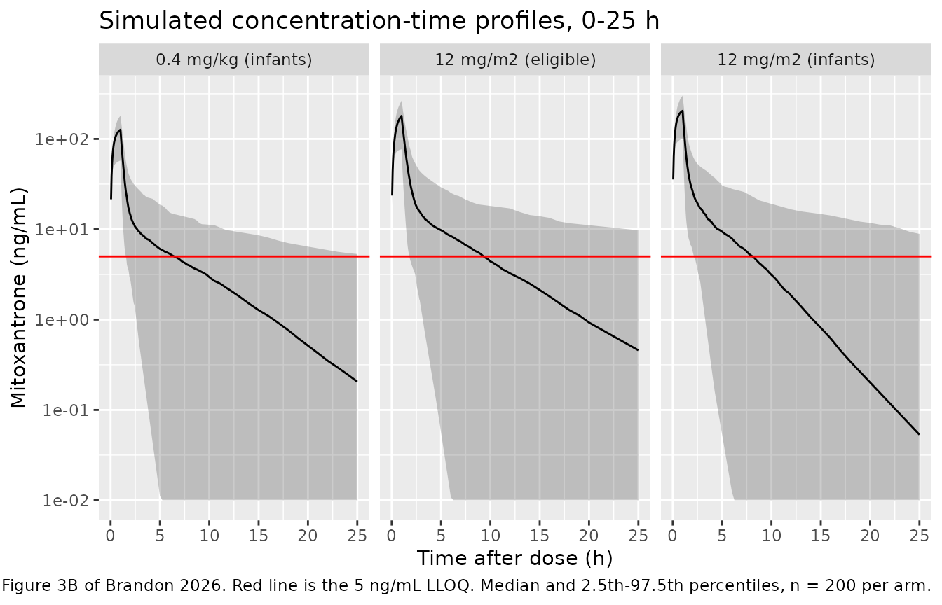
The fraction of simulated observations falling below the LLOQ is a check on the same structure Figure 3C displays as a probability curve. The paper’s modelled dataset was 45.7% below the limit, over a sampling schedule that deliberately reached 72 h past the last dose.
blq <- sim |>
  dplyr::filter(time > 0) |>
  dplyr::group_by(treatment) |>
  dplyr::summarise(`% below LLOQ` = round(100 * mean(Cc < 5), 1), .groups = "drop")
knitr::kable(blq, caption = "Simulated observations below the 5 ng/mL LLOQ over the 0-72 h grid.")| treatment | % below LLOQ |
|---|---|
| 0.4 mg/kg (infants) | 50.2 |
| 12 mg/m2 (eligible) | 43.2 |
| 12 mg/m2 (infants) | 44.2 |
PKNCA validation
sim_nca <- sim |>
  dplyr::filter(!is.na(Cc)) |>
  # Per subject, keep Cc >= 1e-6 * Cmax after the peak: below that the ODE integrator has no relative accuracy left.
  dplyr::group_by(id) |>
  dplyr::filter(time <= time[which.max(Cc)] | Cc >= 1e-6 * max(Cc)) |>
  dplyr::ungroup() |>
  dplyr::select(id, time, Cc, treatment)

# Guarantee a time = 0 row per subject so PKNCA can anchor AUC from 0. The dose
# is an infusion, so the pre-dose concentration is 0.
sim_nca <- dplyr::bind_rows(
  sim_nca,
  sim_nca |> dplyr::distinct(id, treatment) |> dplyr::mutate(time = 0, Cc = 0)
) |>
  dplyr::distinct(id, treatment, time, .keep_all = TRUE) |>
  dplyr::arrange(id, treatment, time)

dose_df <- events |>
  dplyr::filter(evid == 1) |>
  dplyr::select(id, time, amt, treatment)

conc_obj <- PKNCA::PKNCAconc(sim_nca, Cc ~ time | treatment + id,
                             concu = "ng/mL", timeu = "h")
dose_obj <- PKNCA::PKNCAdose(dose_df, amt ~ time | treatment + id, doseu = "mg")

intervals <- data.frame(
  start = 0, end = Inf,
  cmax = TRUE, tmax = TRUE, aucinf.obs = TRUE, half.life = TRUE
)

nca_res <- PKNCA::pk.nca(PKNCA::PKNCAdata(conc_obj, dose_obj, intervals = intervals))

nca_tbl <- as.data.frame(nca_res$result) |>
  dplyr::filter(PPTESTCD %in% c("cmax", "tmax", "aucinf.obs", "half.life"))
stopifnot(nrow(nca_tbl) > 0, !anyNA(nca_tbl$PPORRES))
AUCinf from NCA reproduces Dose / CL per subject
This is the cohort-level version of the deterministic check above, and it is the link between the packaged ODE and the exposure metric the paper actually reports. Both sides use the same drawn clearances, so the difference is pure numerical error and a tight bound is appropriate.
cl_i <- sim |> dplyr::distinct(id, treatment, cl)
dose_i <- dose_df |> dplyr::select(id, amt)

auc_cmp <- nca_tbl |>
  dplyr::filter(PPTESTCD == "aucinf.obs") |>
  dplyr::select(id, treatment, auc_nca = PPORRES) |>
  dplyr::left_join(cl_i, by = c("id", "treatment")) |>
  dplyr::left_join(dose_i, by = "id") |>
  dplyr::mutate(auc_closed = amt / cl * 1000,
                pct_diff   = 100 * (auc_nca - auc_closed) / auc_closed)

cat(sprintf("AUCinf vs Dose/CL across %d subjects: median %+.3f%%, max |diff| %.3f%%\n",
            nrow(auc_cmp), median(auc_cmp$pct_diff), max(abs(auc_cmp$pct_diff))))
#> AUCinf vs Dose/CL across 600 subjects: median -0.032%, max |diff| 0.262%
stopifnot(max(abs(auc_cmp$pct_diff)) < 1)
Exposure by dosing group (replicates Figure 4)
auc_by_arm <- auc_cmp |>
  dplyr::mutate(treatment = factor(treatment, levels = vapply(arm_spec, `[[`, character(1), "label")))

ggplot(auc_by_arm, aes(treatment, auc_nca)) +
  geom_boxplot(outlier.alpha = 0.3) +
  scale_y_log10() +
  labs(x = NULL, y = "AUCinf (mcg*h/L)",
       title = "Simulated mitoxantrone exposure by dosing regimen",
       caption = paste("Replicates Figure 4 of Brandon 2026: infants eligible for",
                       "0.4 mg/kg dosing, the same infants given 12 mg/m2, and",
                       "children eligible for 12 mg/m2. 1 mcg*h/L = 1 ng*h/mL."))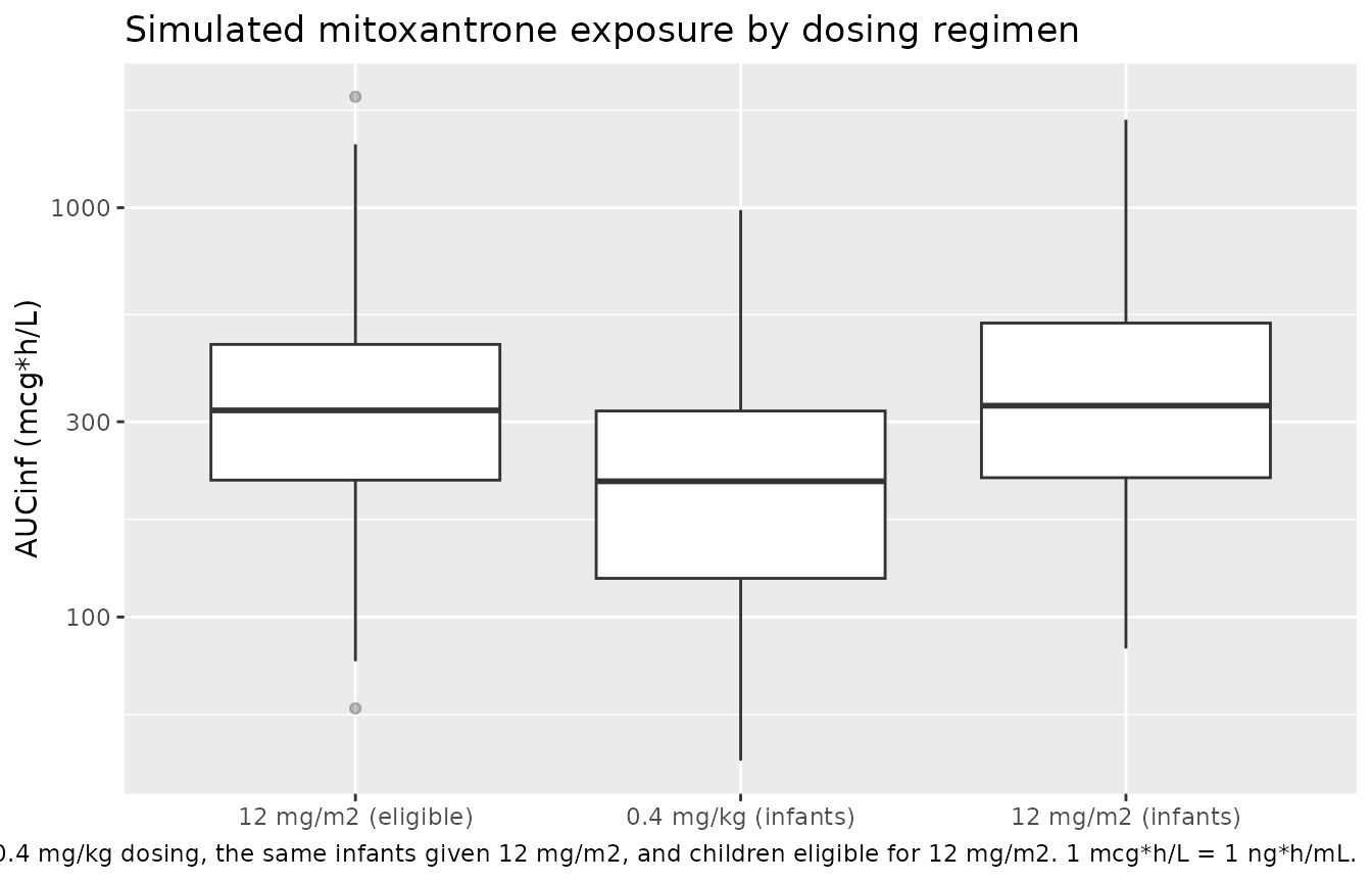
Comparison against the published exposures
The paper reports exposure as mean +/- SD, so the simulated side is pre-aggregated to the mean rather than left to the default median.
sim_wide <- auc_by_arm |>
  dplyr::group_by(treatment) |>
  dplyr::summarise(aucinf.obs = mean(auc_nca), .groups = "drop") |>
  as.data.frame()

# Brandon 2026 Results 3.4, the 1000-virtual-patient simulation underlying
# Figure 4.
published <- data.frame(
  treatment  = vapply(arm_spec, `[[`, character(1), "label"),
  aucinf.obs = c(388, 234, 365)
)

cmp <- nlmixr2lib::ncaComparisonTable(
  simulated = sim_wide, reference = published,
  by = "treatment",
  units = c(aucinf.obs = "mcg*h/L"),
  tolerance_pct = 20
)

knitr::kable(cmp, caption = paste(
  "Mean simulated AUCinf vs. the values reported in Brandon 2026 Results 3.4.",
"* differs from the reference by more than 20%."))| NCA parameter | treatment | Reference | Simulated | % diff |
|---|---|---|---|---|
| AUC0-∞ (obs) (mcg*h/L) | 12 mg/m2 (eligible) | 388 | 379 | -2.3% |
| AUC0-∞ (obs) (mcg*h/L) | 0.4 mg/kg (infants) | 234 | 242 | +3.6% |
| AUC0-∞ (obs) (mcg*h/L) | 12 mg/m2 (infants) | 365 | 391 | +7.0% |
# A loose gate only. The reference is a mean of a heavy-tailed 1/lognormal over
# a covariate pool this vignette cannot reproduce, and the simulated mean over
# 200 subjects carries roughly 6% Monte Carlo error on top. 35% still goes red
# on a mis-transcribed clearance, dose or unit, which move exposure by tens of
# percent; the structural gates below are the ones with real teeth.
stopifnot(max(abs(as.numeric(gsub("[^0-9.+-]", "", cmp[["% diff"]])))) < 35)
The paper’s dosing conclusions
Two claims carry the paper: that infants on the reduced body-weight-based regimen are under-exposed relative to children on the standard regimen, and that a standardised 12 mg/m^2 regimen “would likely result in comparable AUCs across all ages” (Abstract, Results 3.4). Both are ratios between arms, so they are far more robust to the unpublished covariate pool than the absolute means above are, and both are asserted on medians rather than means.
The structural reason the second claim holds is visible in the model:
exposure under BSA-based dosing goes as BSA / WT^0.75, and
the Table 1 BSA relation is WT^0.731 – so the weight
dependence very nearly cancels.
med <- auc_by_arm |>
  dplyr::group_by(treatment) |>
  dplyr::summarise(median_auc = median(auc_nca), .groups = "drop")

m <- stats::setNames(med$median_auc, as.character(med$treatment))

claims <- data.frame(
  Claim = c(
    "Infants on 0.4 mg/kg are under-exposed vs children on 12 mg/m2",
    "Standardised 12 mg/m2 gives comparable exposure across ages",
    "Switching infants from 0.4 mg/kg to 12 mg/m2 raises exposure"
  ),
  Achieved = c(
    sprintf("%.0f%% of the 12 mg/m2 median",  100 * m[["0.4 mg/kg (infants)"]] / m[["12 mg/m2 (eligible)"]]),
    sprintf("%+.0f%% vs the 12 mg/m2 median", 100 * (m[["12 mg/m2 (infants)"]] / m[["12 mg/m2 (eligible)"]] - 1)),
    sprintf("%.2f-fold",                      m[["12 mg/m2 (infants)"]] / m[["0.4 mg/kg (infants)"]])
  )
)
knitr::kable(claims, caption = "The paper's dosing conclusions, reproduced from the packaged model.")| Claim | Achieved |
|---|---|
| Infants on 0.4 mg/kg are under-exposed vs children on 12 mg/m2 | 67% of the 12 mg/m2 median |
| Standardised 12 mg/m2 gives comparable exposure across ages | +3% vs the 12 mg/m2 median |
| Switching infants from 0.4 mg/kg to 12 mg/m2 raises exposure | 1.53-fold |
stopifnot(
  # Under-exposure: at least 20% below. Driven by the dose ratio, not by a draw.
  m[["0.4 mg/kg (infants)"]] < 0.80 * m[["12 mg/m2 (eligible)"]],
  # Comparable across ages: within 25%. The near-cancellation above makes the
  # true value a few percent; 25% leaves room for cohort noise while still
  # going red if the allometric exponent or the BSA relation is wrong.
  abs(m[["12 mg/m2 (infants)"]] / m[["12 mg/m2 (eligible)"]] - 1) < 0.25,
  # Switching raises exposure. Paper's own simulated ratio was 365/234 = 1.56.
  m[["12 mg/m2 (infants)"]] / m[["0.4 mg/kg (infants)"]] > 1.3
)
Assumptions and deviations
-
Body-surface-area relation. The model itself uses
only body weight, but the 12 mg/m^2 dose requires BSA. The paper
publishes no height-based BSA formula and no per-patient heights, so
BSA = 0.0878 * WT^0.731was recovered from the weight / BSA median pairs of Table 1 and verified against all three of them (within 2.5%) before use. Any BSA formula that reproduces those medians gives the same conclusions, because the dosing claims above depend on the BSA-to-weight exponent rather than on the constant. - Infant weight distribution. The paper’s simulations resampled real covariate combinations from a 442-patient cohort aged 1 day to 18 years, which is not published. The infant arms here sample body weight log-uniformly from 3.3 kg (a term newborn) to the 10 kg eligibility ceiling. This affects the absolute means in the comparison table; it largely cancels from the between-arm ratios, which is why the gated claims are ratios.
-
Exposure metric. The paper computes
AUC = Dose / CL_ifrom post hoc Bayesian clearances rather than by NCA. This vignette computes AUCinf by PKNCA from the simulated profiles and shows the two agree to better than 1% per subject, then uses the NCA values throughout. -
Post hoc versus prior draws. The observed-cohort
exposures in Results 3.3 (317 +/- 184 mcg*h/L for the mg/m^2 group) come
from post hoc clearances, which are shrunk toward the typical value (CL
eta-shrinkage 10.65%). The cohort here draws clearances from the full
prior, so its mean sits above the typical-value exposure by roughly
exp(omega^2 / 2)= 1.19. The comparison table above therefore uses the Results 3.4 simulation values, which are generated the same way this vignette’s are, rather than the Results 3.3 observed values. -
Residual error is not exercised by the exposure
checks.
Ccis the individual prediction; theadd(2.5) + prop(0.382)residual appears in thesimcolumn. Exposure comparisons deliberately useCc, matching the paper. - Below-LLOQ handling. The paper fit with the likelihood-based M3 method because 45.7% of its observations were below 5 ng/mL. Simulation has no equivalent step – the model emits continuous concentrations – so the below-LLOQ fraction reported above is descriptive only and is not a reproduction of Figure 3C.
- No exposure-response model. The paper’s title mentions dose-response relationships, but the analysis found “no correlation … between severe (grade 3-4) toxicity, AUC or CL” and reported no statistically significant effect of dosing regimen or concomitant cytarabine (Results 3.3, Supporting Information Tables S2 and S3). There is no fitted exposure-response model to extract, so this package contains only the popPK model.
-
Covariates screened but not retained. BSA, age,
total bilirubin and ALT were tested and rejected (Methods 2.3, Results
3.2); sex, height, serum creatinine, eGFR and serum albumin were carried
in the analysis dataset and plotted in Supporting Information Figure S1
but are not reported as tested on any PK parameter. All are recorded in
the model file’s
covariatesDataExcludedmetadata rather than incovariateData. -
Vc is not an estimate.
lvcis fixed at 23.2 L, the value O’Brien 2010 reported in a comparable paediatric cohort, “to improve model stability” (Results 3.2). The paper notes that estimating it “did not produce any notable change in final estimates but reduced model stability between repeated runs”.