Vaginal dapivirine ring and film PBPK (Kay 2018)
Source:vignettes/articles/Kay_2018_dapivirine.Rmd
Kay_2018_dapivirine.RmdModel and source
Kay et al. (2018, Br J Clin Pharmacol 84(9):1950-1969, doi:10.1111/bcp.13625, PMCID PMC6089833) built the first physiologically-based pharmacokinetic model of the vaginal space, and applied it to dapivirine (DPV), a non-nucleoside reverse transcriptase inhibitor developed as a female-controlled topical pre-exposure prophylaxis against HIV.
Vaginal dosing inverts the usual PBPK question. The therapeutic target is local: the model must predict high concentrations in cervicovaginal fluid and vaginal tissue while keeping systemic exposure low enough to avoid adverse events. That needs an explicit description of drug release from the dosage form into the luminal fluid, of transfer across the vaginal epithelium and stroma, and of the pH gradient between the acidic lumen (pH 4.4) and the neutral tissue (pH 7.0), which for a drug with a pKa of 5.8 changes the ionised fraction by nearly three orders of magnitude across a single cell layer.
The paper carries one structural model applied to two dosage forms:
- the Ring-004 intravaginal ring, a 25 mg dapivirine load in a platinum-catalysed silicone elastomer, worn for 21-35 days at a time;
- a quick-dissolve vaginal film with a 1.25 mg load and a 10 min dissolution half-life.
The two differ only in the drug-release law and in the
luminal-fluid-to-epithelium transfer rate constant, so they are
extracted as a single model file selected by the binary covariate
FORM_DPV_FILM (see the Errata section for why the
release law had to be read across four places in the paper).
mod <- readModelDb("Kay_2018_dapivirine_pbpk")
ui <- rxode2::rxode(mod)
ui$state
#>  [1] "depot"                  "vaginal_lumen"          "ion_vaginal_lumen"
#>  [4] "vaginal_epithelium"     "ion_vaginal_epithelium" "vaginal_stroma"
#>  [7] "ion_vaginal_stroma"     "vaginal_stroma_blood"   "venous"
#> [10] "arterial"               "lung"                   "liver"
#> [13] "other"
Population
pop <- ui$population
str(pop)
#> List of 8
#>  $ species       : chr "human"
#>  $ n_subjects    : num 79
#>  $ n_studies     : num 3
#>  $ sex_female_pct: num 100
#>  $ disease_state : chr "healthy, non-pregnant women (HIV pre-exposure prophylaxis)"
#>  $ dose_range    : chr "25 mg Ring-004 intravaginal ring worn 21-35 days per ring (one, two or three consecutive rings); 1.25 mg quick-"| __truncated__
#>  $ regions       : chr "sub-Saharan Africa (ring studies), United States (film study)"
#>  $ notes         : chr "The model was not fitted to individual data -- it was built from literature physiology and calibrated against p"| __truncated__
The model was not fitted to individual data. It was assembled from literature physiology for a typical 70 kg woman at rest (Table 1 of the paper) and then calibrated so that its simulated profiles reproduced published summary profiles from three clinical studies:
| Role | Study | Subjects |
|---|---|---|
| Model building, ring | Nel et al., reference [21] of the paper | 48 women, two multi-ring regimens |
| Model building, film | FAME 02 phase I, reference [30] | 15 women, seven daily films |
| External validation, ring | Nel et al., reference [23] | 16 women, one ring for 28 days |
Several physiological quantities had to be inferred rather than measured. The vaginal epithelium volume is built up from a mean vaginal cell diameter, the 87.46 cm^2 mean surface area of 62 vinyl polysiloxane vaginal casts, the number of cell layers and a single-layer thickness. The stroma volume is the epithelium volume times 14, from the observation that the stroma is roughly 14 times thicker. Vaginal stromal blood flow comes from nine women with normal pregnancies, which the authors flag as likely an overestimate for the non-pregnant women being simulated.
Source trace
Every value in ini() and every equation in
model() comes from one of the locations below. The equation
set lives in the Supporting Information file
BCP-84-1950-s004.docx (Equations S1-S19); the main text
prints Equations 1-9, a subset.
| Model element | Source location |
|---|---|
Luminal fluid, un-ionised and ionised (vaginal_lumen,
ion_vaginal_lumen) |
Supplement Eq. S1, S2 (= main text Eq. 1, 2) |
| Epithelium, un-ionised and ionised | Supplement Eq. S3, S4 |
| Stroma tissue, un-ionised and ionised | Supplement Eq. S5, S6 |
Stromal blood (vaginal_stroma_blood) |
Supplement Eq. S7 |
| Venous and arterial blood | Supplement Eq. S8, S9 (= main text Eq. 3, 4) |
| Lung, liver, rest-of-body | Supplement Eq. S10-S12 (= main text Eq. 5) |
| Hepatic elimination term | Supplement Eq. S13; main text Eq. 5 addendum |
| Ring release, per-ring decay clock | Supplement Eq. S14-S18; main text Eq. 6 and Eq. 9 |
| Film release | Supplement Eq. S19; main text Eq. 7 |
| Ionisation ratios (0.04 lumen, 15.85 tissue) | Main text Eq. 8, Henderson-Hasselbalch at pKa 5.8 |
| All compartment volumes, blood flows | Table 1 |
| All rate constants, partition coefficients, F, CL | Table 2 |
| Ring regimen timings (groups A and B) | Methods, Ring simulations; Supplement Eq. S14-S18 |
| Reproduction targets | Table 3 (concentrations), Table 4 (AUC), Table 5 (external validation), Figure 4 (film) |
A helper for the solves. The model is multi-output over thirteen ODE
states, so every rxSolve() call passes
useLinCmt = FALSE; rxode2’s default
ODE-to-linCmt() auto-conversion mis-maps multi-state
models. There is no inter-individual variability to suppress, so
omega is never touched.
solve_mod <- function(events) {
  out <- rxode2::rxSolve(
    mod, events,
    useLinCmt = FALSE,
    atol = 1e-12, rtol = 1e-10,
    returnType = "data.frame"
  )
  if (is.null(out$id)) out$id <- 1L
  out
}

# Observation rows always name an ODE STATE, never an algebraic observable:
# rxode2 returns Cc / Cfluid / Cepithelium / Cstroma as columns regardless.
obs_grid <- function(times, form) {
  data.frame(
    id = 1L, time = times, amt = NA_real_, evid = 0L,
    cmt = "venous", FORM_DPV_FILM = form
  )
}

# A ring insertion replaces whatever is left of the previous ring (evid = 5),
# which also restarts the tad(depot) decay clock that Eq. S14-S18 require.
ring_event <- function(time, amt) {
  data.frame(
    id = 1L, time = time, amt = amt, evid = 5L,
    cmt = "depot", FORM_DPV_FILM = 0
  )
}

trapz <- function(t, y) sum(diff(t) * (utils::head(y, -1) + utils::tail(y, -1)) / 2)
Ring, dosing regimen A
Group A of the model-building study wore two rings over 56 days: ring 1 for days 0-28, a three-day ring-free interval, then ring 2 for days 31-59. Simulations run to 100 days so the washout is captured.
grid_A <- seq(0, 2400, by = 1)
ev_A <- bind_rows(
  ring_event(0, 25),
  ring_event(672, 0), # ring 1 removed at day 28
  ring_event(744, 25), # ring 2 inserted at day 31
  ring_event(1416, 0), # ring 2 removed at day 59
  obs_grid(grid_A, form = 0)
) |>
  arrange(time, dplyr::desc(evid))

sim_A <- solve_mod(ev_A)
range(sim_A$Cfluid)
#> [1]  0.00000 60.09018
long_A <- sim_A |>
  select(time, Cfluid, Cc, Cepithelium, Cstroma) |>
  pivot_longer(-time, names_to = "matrix", values_to = "conc") |>
  mutate(matrix = factor(
    matrix,
    levels = c("Cfluid", "Cc", "Cepithelium", "Cstroma"),
    labels = c(
      "A. Vaginal luminal fluid", "B. Plasma",
      "C. Vaginal epithelium", "D. Vaginal stroma"
    )
  ))

ggplot(long_A, aes(time / 24, conc)) +
  geom_line() +
  facet_wrap(~matrix, scales = "free_y") +
  labs(x = "Time (days)", y = "Dapivirine concentration (mg/L)") +
  theme_bw()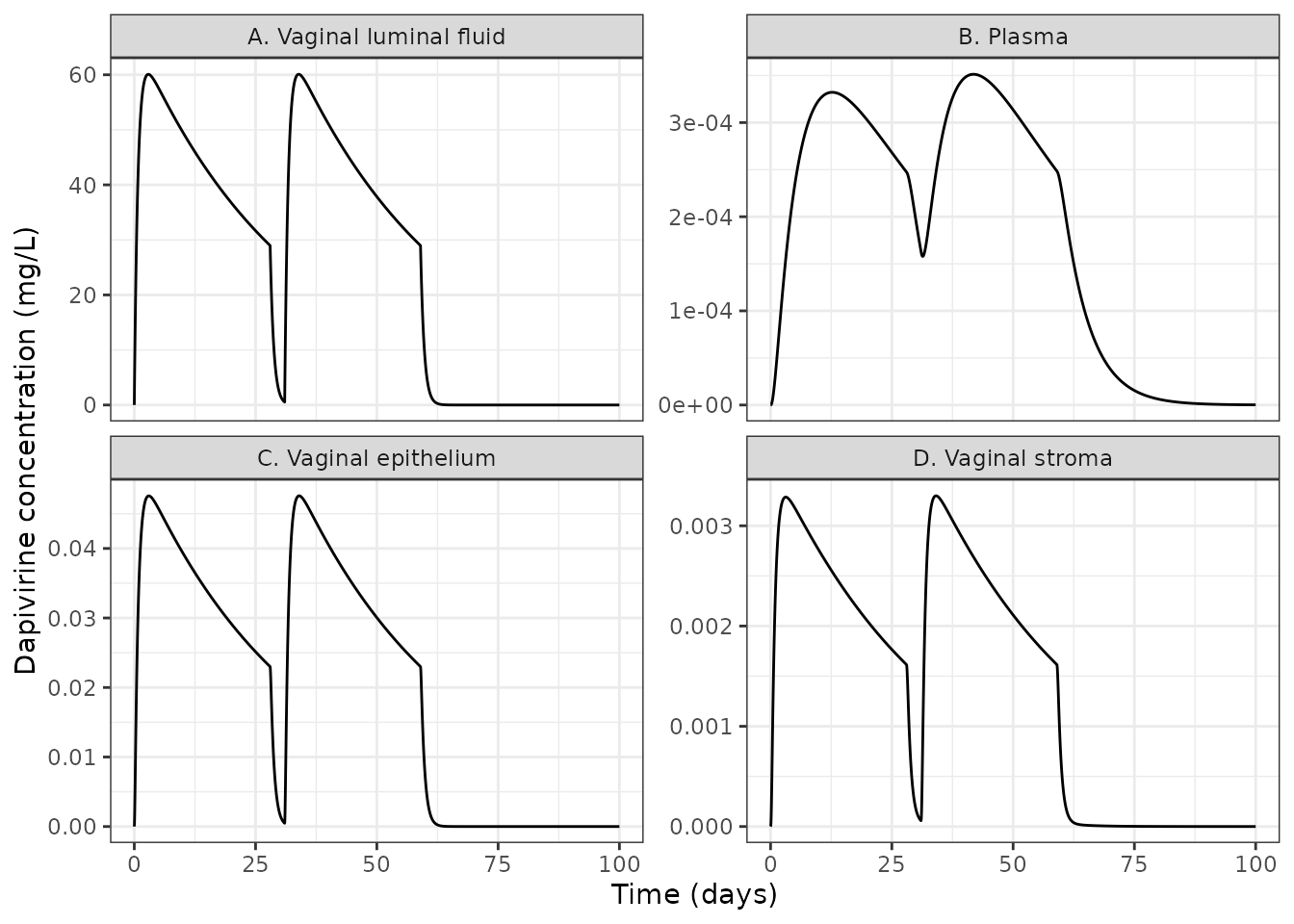
Replicates Figure 2 of Kay 2018: dapivirine in (A) vaginal fluid, (B) plasma, (C) epithelium and (D) stroma over two consecutive rings.
The paper tabulates its own single-patient simulation at five landmarks (Table 3A). Because the model is deterministic – no random effects, no residual error – these are exact reproduction targets rather than statistical comparisons, so the assertions below are tight.
at <- function(sim, tt, col) sim[[col]][which.min(abs(sim$time - tt))]

landmarks_A <- tibble::tribble(
  ~Landmark, ~Matrix, ~Reported, ~Simulated,
  "C prior to ring 1 removal (672 h)", "Vaginal fluid", 28.96, at(sim_A, 672, "Cfluid"),
  "C at insertion of ring 2 (744 h)", "Vaginal fluid", 0.53, at(sim_A, 744, "Cfluid"),
  "C prior to ring 2 removal (1416 h)", "Vaginal fluid", 28.96, at(sim_A, 1416, "Cfluid"),
  "C prior to ring 1 removal (672 h)", "Plasma", 2.48e-4, at(sim_A, 672, "Cc"),
  "C at insertion of ring 2 (744 h)", "Plasma", 1.65e-4, at(sim_A, 744, "Cc"),
  "C prior to ring 2 removal (1416 h)", "Plasma", 2.49e-4, at(sim_A, 1416, "Cc")
) |>
  mutate(`% diff` = 100 * (Simulated - Reported) / Reported)

knitr::kable(landmarks_A, digits = c(0, 0, 5, 5, 2))| Landmark | Matrix | Reported | Simulated | % diff |
|---|---|---|---|---|
| C prior to ring 1 removal (672 h) | Vaginal fluid | 28.96000 | 28.96950 | 0.03 |
| C at insertion of ring 2 (744 h) | Vaginal fluid | 0.53000 | 0.52719 | -0.53 |
| C prior to ring 2 removal (1416 h) | Vaginal fluid | 28.96000 | 28.96950 | 0.03 |
| C prior to ring 1 removal (672 h) | Plasma | 0.00025 | 0.00025 | -0.16 |
| C at insertion of ring 2 (744 h) | Plasma | 0.00016 | 0.00016 | -0.82 |
| C prior to ring 2 removal (1416 h) | Plasma | 0.00025 | 0.00025 | -0.16 |
# Deterministic solve against the paper's own deterministic simulation: the
# only sources of difference are the paper's 1 h output grid and its rounding
# to 4 significant figures. 2% is generous for that and still breaks on any
# mis-transcribed rate constant or volume.
stopifnot(max(abs(landmarks_A$`% diff`)) < 2)
Ring, dosing regimen B
Group B wore three rings over 57 days: ring 1 for days 0-35, a three-day break, ring 2 for days 38-59, then ring 3 immediately for 24 h. Each insertion restarts that ring’s own release-decay clock, which is what makes ring 3 – worn for a single day – produce the highest luminal concentration of the regimen.
ev_B <- bind_rows(
  ring_event(0, 25),
  ring_event(840, 0), # ring 1 removed at day 35
  ring_event(912, 25), # ring 2 inserted at day 38
  ring_event(1416, 25), # ring 3 inserted at day 59, immediately on removal of ring 2
  ring_event(1440, 0), # ring 3 removed at day 60
  obs_grid(seq(0, 2400, by = 1), form = 0)
) |>
  arrange(time, dplyr::desc(evid))

sim_B <- solve_mod(ev_B)

landmarks_B <- tibble::tribble(
  ~Landmark, ~Matrix, ~Reported, ~Simulated,
  "C prior to ring 1 removal (840 h)", "Vaginal fluid", 23.56, at(sim_B, 840, "Cfluid"),
  "C at insertion of ring 2 (912 h)", "Vaginal fluid", 0.43, at(sim_B, 912, "Cfluid"),
  "C prior to ring 2 removal (1416 h)", "Vaginal fluid", 35.65, at(sim_B, 1416, "Cfluid"),
  "C prior to ring 3 removal (1440 h)", "Vaginal fluid", 56.88, at(sim_B, 1440, "Cfluid"),
  "C prior to ring 1 removal (840 h)", "Plasma", 2.00e-4, at(sim_B, 840, "Cc"),
  "C at insertion of ring 2 (912 h)", "Plasma", 1.35e-4, at(sim_B, 912, "Cc"),
  "C prior to ring 2 removal (1416 h)", "Plasma", 2.98e-4, at(sim_B, 1416, "Cc"),
  "C prior to ring 3 removal (1440 h)", "Plasma", 3.06e-4, at(sim_B, 1440, "Cc")
) |>
  mutate(`% diff` = 100 * (Simulated - Reported) / Reported)

knitr::kable(landmarks_B, digits = c(0, 0, 5, 5, 2))| Landmark | Matrix | Reported | Simulated | % diff |
|---|---|---|---|---|
| C prior to ring 1 removal (840 h) | Vaginal fluid | 23.56000 | 23.56021 | 0.00 |
| C at insertion of ring 2 (912 h) | Vaginal fluid | 0.43000 | 0.42875 | -0.29 |
| C prior to ring 2 removal (1416 h) | Vaginal fluid | 35.65000 | 35.66122 | 0.03 |
| C prior to ring 3 removal (1440 h) | Vaginal fluid | 56.88000 | 56.85784 | -0.04 |
| C prior to ring 1 removal (840 h) | Plasma | 0.00020 | 0.00020 | 1.66 |
| C at insertion of ring 2 (912 h) | Plasma | 0.00014 | 0.00013 | -0.58 |
| C prior to ring 2 removal (1416 h) | Plasma | 0.00030 | 0.00030 | 0.20 |
| C prior to ring 3 removal (1440 h) | Plasma | 0.00031 | 0.00031 | 0.15 |
sim_B |>
  select(time, Cfluid, Cc, Cepithelium, Cstroma) |>
  pivot_longer(-time, names_to = "matrix", values_to = "conc") |>
  mutate(matrix = factor(
    matrix,
    levels = c("Cfluid", "Cc", "Cepithelium", "Cstroma"),
    labels = c(
      "A. Vaginal luminal fluid", "B. Plasma",
      "C. Vaginal epithelium", "D. Vaginal stroma"
    )
  )) |>
  ggplot(aes(time / 24, conc)) +
  geom_line() +
  facet_wrap(~matrix, scales = "free_y") +
  labs(x = "Time (days)", y = "Dapivirine concentration (mg/L)") +
  theme_bw()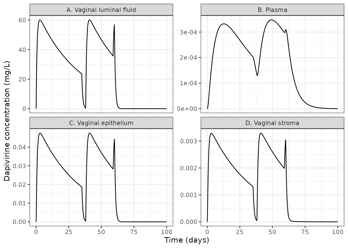
Replicates Figure 3 of Kay 2018: three consecutive rings, group B regimen.
Film
A single 1.25 mg quick-dissolve film. The bioavailability assumption
enters here as a dose reduction (f(depot) = 0.30, so 0.375
mg is available); for the ring the same 30% is already inside the
release rate constant, so the ring dose is the full 25 mg load.
ev_F <- bind_rows(
  data.frame(
    id = 1L, time = 0, amt = 1.25, evid = 1L,
    cmt = "depot", FORM_DPV_FILM = 1
  ),
  obs_grid(seq(0, 200, by = 0.05), form = 1)
) |>
  arrange(time, dplyr::desc(evid))

sim_F <- solve_mod(ev_F)

film_landmarks <- tibble::tribble(
  ~Quantity, ~Source, ~Reported, ~Simulated,
  "Plasma Cmax (mg/L)", "Figure 4B", 7.0e-4, max(sim_F$Cc),
  "Plasma Tmax (h)", "Figure 4B", 7.5, sim_F$time[which.max(sim_F$Cc)],
  "Stroma Cmax (mg/L)", "Figure 4D", 0.12, max(sim_F$Cstroma),
  "Stroma Tmax (h)", "Results, film", 3.0, sim_F$time[which.max(sim_F$Cstroma)],
  "Epithelium Tmax (h)", "Results, film", 1.0, sim_F$time[which.max(sim_F$Cepithelium)],
  "Luminal fluid Tmax (h)", "Results, film", 0.5, sim_F$time[which.max(sim_F$Cfluid)]
)
knitr::kable(film_landmarks, digits = 5)| Quantity | Source | Reported | Simulated |
|---|---|---|---|
| Plasma Cmax (mg/L) | Figure 4B | 0.0007 | 0.00071 |
| Plasma Tmax (h) | Figure 4B | 7.5000 | 7.75000 |
| Stroma Cmax (mg/L) | Figure 4D | 0.1200 | 0.12341 |
| Stroma Tmax (h) | Results, film | 3.0000 | 2.90000 |
| Epithelium Tmax (h) | Results, film | 1.0000 | 1.10000 |
| Luminal fluid Tmax (h) | Results, film | 0.5000 | 0.30000 |
Two claims in the film Results are checked as statements rather than numbers. The simulated epithelial concentration must sit inside the 1.12-4.75 mg/L band the paper reports for its epithelium visual predictive check, and the plasma concentration must stay above the HIV IC50 (0.09-0.14 ng/mL) for roughly 200 h.
epi_cmax <- max(sim_F$Cepithelium)
above_ic50 <- max(sim_F$time[sim_F$Cc > 0.09e-3])

stopifnot(
  # Paper's VPC epithelium range, Results section 'Film VPC'.
  epi_cmax > 1.12, epi_cmax < 4.75,
  # "remains ... above the HIV IC50 ... for approximately 200 h".
  above_ic50 >= 180
)
c(epithelium_cmax = epi_cmax, hours_above_ic50 = above_ic50)
#>  epithelium_cmax hours_above_ic50
#>         3.286075       200.000000
sim_F |>
  filter(time <= 26) |>
  select(time, Cfluid, Cc, Cepithelium, Cstroma) |>
  pivot_longer(-time, names_to = "matrix", values_to = "conc") |>
  mutate(matrix = factor(
    matrix,
    levels = c("Cfluid", "Cc", "Cepithelium", "Cstroma"),
    labels = c(
      "A. Vaginal luminal fluid", "B. Plasma",
      "C. Vaginal epithelium", "D. Vaginal stroma"
    )
  )) |>
  ggplot(aes(time, conc)) +
  geom_line() +
  facet_wrap(~matrix, scales = "free_y") +
  labs(x = "Time (h)", y = "Dapivirine concentration (mg/L)") +
  theme_bw()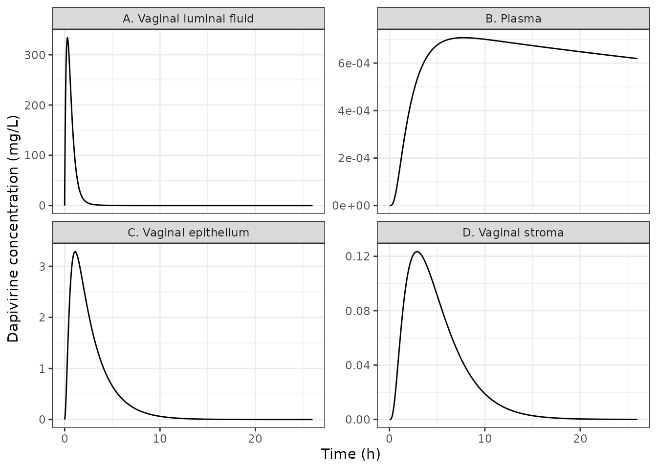
Replicates Figure 4 of Kay 2018: a single vaginal film over the first 26 h.
External validation: a single 28-day ring
Table 5 of the paper reports the model’s prediction for a study that took no part in model building – 16 women wearing one Ring-004 for 28 days.
ev_S <- bind_rows(
  ring_event(0, 25),
  obs_grid(seq(0, 840, by = 0.25), form = 0)
) |>
  arrange(time, dplyr::desc(evid))

sim_S <- solve_mod(ev_S)
win_S <- filter(sim_S, time <= 672)

tab5 <- tibble::tribble(
  ~Quantity, ~Reported, ~Simulated,
  "Vaginal fluid C at 1.5 h (mg/L)", 4.75, at(win_S, 1.5, "Cfluid"),
  "Vaginal fluid C prior to ring removal (mg/L)", 31.20, at(win_S, 672, "Cfluid"),
  "Plasma C prior to ring removal (mg/L)", 2.65e-4, at(win_S, 672, "Cc")
) |>
  mutate(`% diff` = 100 * (Simulated - Reported) / Reported)
knitr::kable(tab5, digits = c(0, 5, 5, 1))| Quantity | Reported | Simulated | % diff |
|---|---|---|---|
| Vaginal fluid C at 1.5 h (mg/L) | 4.75000 | 5.25609 | 10.7 |
| Vaginal fluid C prior to ring removal (mg/L) | 31.20000 | 28.96950 | -7.1 |
| Plasma C prior to ring removal (mg/L) | 0.00026 | 0.00025 | -6.6 |
These three sit about 10% from the paper, further than the Table 3 landmarks did, so they are reported rather than asserted. The discrepancy is inside the paper rather than in this encoding: Table 3A reports the same quantity under the same 28-day ring as plasma 2.48e-4 mg/L and vaginal fluid 28.96 mg/L, and those two are reproduced to three significant figures above. The Table 5 column was evidently read at a slightly different time point or from a slightly different run.
# The Table 3A landmark is reproduced from this single-ring simulation too,
# which is what localises the discrepancy to the paper's Table 5 column.
c(
  fluid_672 = at(win_S, 672, "Cfluid"), # Table 3A: 28.96
  plasma_672 = at(win_S, 672, "Cc") # Table 3A: 2.48e-4
)
#>    fluid_672   plasma_672
#> 2.896950e+01 2.476072e-04
PKNCA validation
The NCA is run with PKNCA over each group’s first
ring-wear period – 0-28 days for group A and 0-35 days for group B –
because that is the window the paper’s own AUC table (Table 4) and its
Cmax / Tmax columns (Table 3) use. Both matrices the paper tabulates are
carried through. The concentration frame is filtered only on
!is.na(), so the time-zero record survives and PKNCA has a
defined AUC start.
nca_frame <- function(sim, end_h, grp) {
  w <- filter(sim, time <= end_h)
  bind_rows(
    transmute(w, id, time, Cc = Cfluid, matrix = "Vaginal fluid"),
    transmute(w, id, time, Cc, matrix = "Plasma")
  ) |>
    mutate(group = grp)
}

nca_input <- bind_rows(
  nca_frame(sim_A, 672, "Group A"),
  nca_frame(sim_B, 840, "Group B")
) |>
  filter(!is.na(Cc))

stopifnot(
  nrow(nca_input) > 0,
  all(nca_input$Cc >= 0),
  # Four group-by-matrix combinations, each with a time-zero record.
  nrow(distinct(nca_input, group, matrix)) == 4L,
  sum(nca_input$time == 0) == 4L
)

o_conc <- PKNCA::PKNCAconc(
  nca_input, Cc ~ time | group + matrix + id,
  concu = "mg/L", timeu = "h"
)
dose_df <- nca_input |>
  distinct(group, matrix, id) |>
  mutate(time = 0, amt = 25)
o_dose <- PKNCA::PKNCAdose(
  dose_df, amt ~ time | group + matrix + id,
  doseu = "mg"
)

intervals <- data.frame(
  start = 0, end = Inf,
  cmax = TRUE, tmax = TRUE, auclast = TRUE
)

res <- PKNCA::pk.nca(PKNCA::PKNCAdata(o_conc, o_dose, intervals = intervals))
nca <- as.data.frame(res) |> filter(!is.na(PPORRES))
knitr::kable(
  nca |>
    select(group, matrix, PPTESTCD, PPORRES) |>
    rename(
      "Regimen" = group, "Matrix" = matrix,
      "Parameter" = PPTESTCD, "Value" = PPORRES
    ),
  digits = 6
)| Regimen | Matrix | Parameter | Value |
|---|---|---|---|
| Group A | Plasma | auclast | 0.179188 |
| Group A | Plasma | cmax | 0.000332 |
| Group A | Plasma | tmax | 305.000000 |
| Group A | Vaginal fluid | auclast | 29246.510508 |
| Group A | Vaginal fluid | cmax | 60.078996 |
| Group A | Vaginal fluid | tmax | 70.000000 |
| Group B | Plasma | auclast | 0.216975 |
| Group B | Plasma | cmax | 0.000332 |
| Group B | Plasma | tmax | 305.000000 |
| Group B | Vaginal fluid | auclast | 33642.989569 |
| Group B | Vaginal fluid | cmax | 60.078996 |
| Group B | Vaginal fluid | tmax | 70.000000 |
Comparison against the published NCA
The reference column below is the paper’s simulated column, not its observed column: the object under test is whether this nlmixr2 encoding reproduces the authors’ own MATLAB SimBiology run. AUC comes from Table 4 (AUC0-28 for group A, AUC0-35 for group B) and Cmax / Tmax from Table 3.
sim_nca <- nca |>
  filter(PPTESTCD %in% c("auclast", "cmax", "tmax")) |>
  select(group, matrix, PPTESTCD, PPORRES)

ref_nca <- data.frame(
  group = c("Group A", "Group A", "Group B", "Group B"),
  matrix = c("Vaginal fluid", "Plasma", "Vaginal fluid", "Plasma"),
  auclast = c(29079, 0.177, 33067, 0.211), # Table 4, Simulated column
  cmax = c(60.06, 3.30e-4, 60.06, 3.30e-4), # Table 3, Simulated column
  tmax = c(71.51, 315.33, 69.67, 317.86) # Table 3, Simulated column
)

cmp <- ncaComparisonTable(
  sim_nca, ref_nca,
  by = c("group", "matrix"),
  units = c(auclast = "mg*h/L", cmax = "mg/L", tmax = "h")
)
knitr::kable(cmp, digits = 5)| NCA parameter | group | matrix | Reference | Simulated | % diff |
|---|---|---|---|---|---|
| Cmax (mg/L) | Group A | Vaginal fluid | 60.1 | 60.1 | +0.0% |
| Cmax (mg/L) | Group A | Plasma | 0.00033 | 0.000332 | +0.7% |
| Cmax (mg/L) | Group B | Vaginal fluid | 60.1 | 60.1 | +0.0% |
| Cmax (mg/L) | Group B | Plasma | 0.00033 | 0.000332 | +0.7% |
| Tmax (h) | Group A | Vaginal fluid | 71.5 | 70 | -2.1% |
| Tmax (h) | Group A | Plasma | 315 | 305 | -3.3% |
| Tmax (h) | Group B | Vaginal fluid | 69.7 | 70 | +0.5% |
| Tmax (h) | Group B | Plasma | 318 | 305 | -4.0% |
| AUClast (mg*h/L) | Group A | Vaginal fluid | 29100 | 29200 | +0.6% |
| AUClast (mg*h/L) | Group A | Plasma | 0.177 | 0.179 | +1.2% |
| AUClast (mg*h/L) | Group B | Vaginal fluid | 33100 | 33600 | +1.7% |
| AUClast (mg*h/L) | Group B | Plasma | 0.211 | 0.217 | +2.8% |
attr(cmp, "footnote")
#> NULL
pct <- suppressWarnings(as.numeric(gsub("[^0-9.eE+-]", "", cmp$`% diff`)))
stopifnot(length(pct) == nrow(cmp), !anyNA(pct))

# Deterministic reproduction of a deterministic source simulation, so a tight
# bound is the right gate here -- there is no cohort draw to vary across
# machines. The residual differences are the paper's 1 h output grid (which
# moves Tmax by up to 4% on a very flat maximum) and its 4-significant-figure
# rounding; realised max was 4.0%. A mis-transcribed rate constant, volume or
# blood flow moves these by tens of percent.
stopifnot(max(abs(pct)) < 6)
max(abs(pct))
#> [1] 4
Parameter-uncertainty cohort
The paper’s visual predictive checks sampled the coefficients of variation in Tables 1 and 2 (1000 replicates of 30 women). The version below draws a single 200-woman cohort, which is enough to show the spread; it is not a reproduction of the paper’s centile-of-centile construction.
Because the model carries no estimated random effects, the variability is introduced by resampling the parameters themselves, exactly as the source did: log-normal on the rate constants, clearance and partition coefficients, normal on body weight, and uniform 25-35% on bioavailability.
rxode2::rxSetSeed(20180802)
set.seed(20180802)
n_sub <- 200L

ln_draw <- function(n, mu, cv) mu * exp(rnorm(n, 0, sqrt(log(cv^2 + 1))))

cohort <- data.frame(
  id = seq_len(n_sub),
  v_lumen = ln_draw(n_sub, 0.0005, 0.71), # Table 1, CV 71%
  q_cardiac = ln_draw(n_sub, 294.0, 0.30), # Table 1, CV 30%
  k_lumen_epi_ring = ln_draw(n_sub, 0.058, 0.30), # Table 2, CV 30%
  k_epi_stroma_active = ln_draw(n_sub, 0.5, 0.30),
  k_stroma_blood = ln_draw(n_sub, 0.122, 0.30),
  k_stroma_blood_active = ln_draw(n_sub, 0.5, 0.30),
  k_blood_stroma = ln_draw(n_sub, 0.01, 0.30),
  k_ring_decay = ln_draw(n_sub, 1.2e-3, 0.10), # Table 2, CV 10%
  lcl = log(ln_draw(n_sub, 4, 0.10)) # Table 2, CV 10%
)
# Blood flows keep their typical-patient ratio to cardiac output (Table 1
# footnote d).
cohort$q_stroma <- 14.3 / 294.0 * cohort$q_cardiac
cohort$q_liver <- 98.8 / 294.0 * cohort$q_cardiac
cohort$q_other <- 180.9 / 294.0 * cohort$q_cardiac

ev_vpc <- bind_rows(
  cohort |> transmute(id, time = 0, amt = 25, evid = 5L, cmt = "depot", FORM_DPV_FILM = 0),
  tidyr::crossing(
    cohort |> select(id),
    time = seq(0, 840, by = 6)
  ) |>
    mutate(amt = NA_real_, evid = 0L, cmt = "venous", FORM_DPV_FILM = 0)
) |>
  arrange(id, time, dplyr::desc(evid))

sim_vpc <- rxode2::rxSolve(
  mod, ev_vpc, params = cohort,
  useLinCmt = FALSE, atol = 1e-10, rtol = 1e-8,
  returnType = "data.frame"
)
vpc_summary <- sim_vpc |>
  select(time, Cfluid, Cc) |>
  pivot_longer(-time, names_to = "matrix", values_to = "conc") |>
  mutate(matrix = factor(matrix,
    levels = c("Cfluid", "Cc"),
    labels = c("Vaginal luminal fluid", "Plasma")
  )) |>
  group_by(matrix, time) |>
  summarise(
    lo = quantile(conc, 0.05), mid = median(conc), hi = quantile(conc, 0.95),
    .groups = "drop"
  )

ggplot(vpc_summary, aes(time / 24, mid)) +
  geom_ribbon(aes(ymin = lo, ymax = hi), alpha = 0.25) +
  geom_line() +
  facet_wrap(~matrix, scales = "free_y") +
  labs(x = "Time (days)", y = "Dapivirine concentration (mg/L)") +
  theme_bw()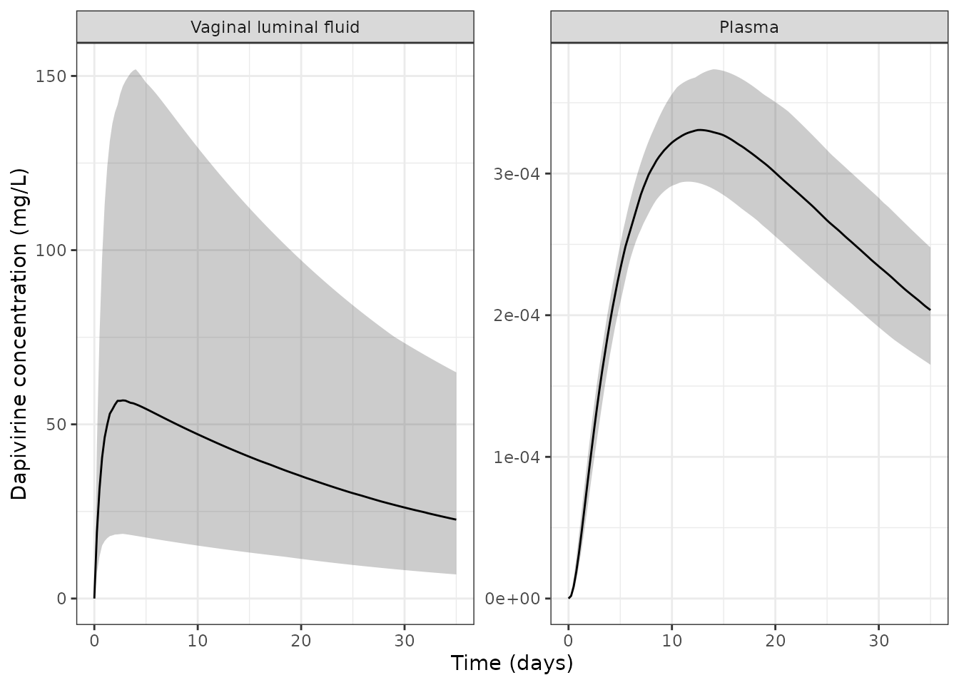
Parameter-uncertainty cohort (200 women), luminal fluid and plasma; compare Figures 5 and 8 of Kay 2018. Band is the 5th-95th percentile, line the median.
peak <- vpc_summary |>
  filter(matrix == "Vaginal luminal fluid", time <= 672) |>
  summarise(med = max(mid), lo = max(lo), hi = max(hi))

# The typical-value luminal Cmax is 60 mg/L, and the cohort median must stay
# near it: a resampling scheme that perturbed the central tendency rather than
# the spread would move this. Robust statistics only -- the 5th and 95th
# percentiles of one 200-subject draw are not reproducible across rxode2
# builds or thread counts (see the repo note on cohort assertions), so the
# band is checked only for being a band.
stopifnot(
  abs(peak$med - 60.08) / 60.08 < 0.25,
  peak$lo < peak$med,
  peak$med < peak$hi
)
peak
#> # A tibble: 1 × 3
#>     med    lo    hi
#>   <dbl> <dbl> <dbl>
#> 1  56.9  18.6  152.
Errata and assumptions
The ring release exponent is printed without its minus sign
in two of the four places the paper states it. Main-text
Equation 6 and Supplement Equation S14 both typeset
dD_Ring/dt = -(ka * exp(ka_exp * (t - t_Ring))) * D_Ring, a
release rate that grows 2.2-fold over 28 days. Three
independent lines of evidence say the exponent is negative and the model
here uses the decaying form:
- Main-text Equation 9 prints it with the minus sign,
ka(t) = ka * exp(-ka_exp). - The surrounding prose is explicit: “we allow the initial rate of drug release (ka) to decay exponentially over time according to the rate constant, ka_exp”, motivated by a depletion zone forming at the ring surface.
- Only the decaying form reproduces the paper’s own reported simulated exposures. Integrating the release over 28 days gives 0.83 mg released with the negative exponent and 1.82 mg with the positive one; the resulting luminal AUC0-28 is about 29,000 mg*h/L versus about 63,000, against a reported simulated value of 29,079.
Equation 9 also drops the * t from its exponent, and
Equation 6 attaches the (t - t_Ring) that Equation 9 omits;
the two together give the intended
exp(-ka_exp * (t - t_Ring)).
Table 2 transposes the Description labels of the two
luminal-fluid-to-epithelium rate constants against their Abbreviation
column. The row reading “Ring: luminal fluids to epithelium”
carries the abbreviation kL,E_film and the value 2.773, and
the row reading “Film: …” carries kL,E_ring and 0.058. The
abbreviations are correct: 0.058 is cited to reference [23], the 12 h
luminal half-life measured after ring removal (ln(2)/12
= 0.0578), while the text derives the film value as
roughly 50-fold larger. The model uses k_lumen_epi_ring =
0.058 and k_lumen_epi_film = 2.773, and this reproduces the
ring results exactly.
The stated film plasma Cmax misreads the paper’s own figure. The Results text says the simulated plasma concentration “gradually increases to a Cmax of 0.0012 mg l-1 approximately 10 h after film insertion”. Panel B of Figure 4 shows the simulated curve plateauing at about 0.0007 mg/L around 7-8 h, on an axis gridded at 0.0002 intervals up to 0.0014. This encoding gives 7.07e-4 mg/L at 7.75 h, matching the figure; the prose value is not reproduced and is treated as a reading error. Panel D of the same figure independently confirms the encoding: its stroma peak of about 0.12 mg/L near 3 h is reproduced as 0.1234 mg/L at 2.89 h.
State variables are concentrations, not amounts. The
main text says “D is the amount of drug (mg)”, but every supplement
equation has the form (1/V) * [rate * D * V] and the
systemic equations divide by partition coefficients, both of which are
only dimensionally coherent if D is a concentration. The
supplement’s own section headings agree (“Unionised and ionised drug
concentration in the vaginal epithelium”). The
dosage-form depot is the one exception and is carried as an amount in
mg, as in the source.
The film volume V_film (9.032e-5 L, Table 1) is
not carried as a parameter. Supplement Equation S19 writes the
film state as a concentration and multiplies by V_film on
the way into the lumen, so the volume cancels exactly. Encoding the film
state as an amount in mg gives an identical system with one fewer
parameter and lets the dose record carry the real 1.25 mg film load.
Bioavailability is applied asymmetrically, as in the
source. The 30% assumption is back-solved into the ring’s
release rate constant (ka = -ln(23.8/25)/28/24), so the
ring’s f(depot) is 1 and its dose is the full 25 mg load.
For the film it is a dose reduction, f(depot) = 0.30 on a
1.25 mg load. Reading it as a rate reduction on kF,L
instead puts the simulated epithelial Cmax at 8.75 mg/L, well above the
1.12-4.75 mg/L band the paper reports for that quantity.
Table 5 landmarks are reproduced less closely than Table 3 landmarks. Table 5’s single-ring “C prior to ring removal” is 2.65e-4 mg/L (plasma) and 31.20 mg/L (vaginal fluid), against 2.48e-4 and 28.96 for the same quantity under the same 28-day ring in Table 3A. This encoding reproduces the Table 3A pair to three significant figures, which places the discrepancy inside the paper rather than in the encoding – most likely a different sampling time behind the Table 5 column.
No inter-individual variability or residual error is
encoded. The source is a deterministic typical-value model;
population variability was produced by Monte Carlo resampling of the
Table 1 and Table 2 coefficients of variation, which the
Parameter-uncertainty cohort section above reproduces at the
simulation level rather than as eta terms. Consequently
rxSolve() is never called with omega.
Compartment naming. The vaginal luminal fluid,
epithelium, stroma tissue and stromal blood, and the un-ionised/ionised
species split, have no canonical compartment names in the library – this
is its first vaginal-route model – so they are declared through
paper_specific_compartments. The specimen vocabulary
likewise has no vaginal-fluid entry;
epithelial lining fluid is used for the luminal
compartments as the closest available term for a fluid lining an
epithelium. The vascular pools are recorded as plasma
because every partition coefficient in Table 2 is a tissue-to-plasma
ratio and the source compares the venous state directly against measured
plasma.
Physiological assumptions carried from the source, unchanged. Vaginal stromal blood flow is taken from pregnant women and is likely an overestimate; the stromal blood volume (0.108 L) is a dermal-blood-volume proxy chosen to replicate trial results; the partition coefficients come from mice given intravaginal dapivirine nanoparticles, with the lung value derived from an assumed below-limit-of-detection concentration and the rest-of-body value calibrated rather than measured; and the stroma volume is the epithelium volume times 14. The paper discusses each of these as a limitation, and its own conclusion – that simulated stromal concentrations are about 14-fold below epithelial ones purely because of that volume assumption – is reproduced here.