Linezolid (Nguyen 2026)
Source:vignettes/articles/Nguyen_2026_linezolid.Rmd
Nguyen_2026_linezolid.RmdModel and source
- Citation: Nguyen TA, Nguyen TP, Nguyen AT, Dinh LV, Nguyen HB, Vu HD, Nguyen TNB, Vu D, Fox GJ, Alffenaar JC, Stocker SL. Single Saliva Sample Linezolid Dosing for Multidrug-Resistant Tuberculosis: A Population Pharmacokinetic Modelling of Plasma and Saliva. Clin Pharmacokinet. 2026;65(5):719-730. doi:10.1007/s40262-026-01626-4.
- Description: One-compartment oral population PK model for linezolid in Vietnamese adults treated for multidrug-resistant tuberculosis (Nguyen 2026), fitted jointly to paired plasma and saliva concentrations. Saliva is carried as a kinetically distinct hypothetical effect compartment driven by the central compartment through a secretion rate constant (kin_saliva = 4.93 1/h), with reabsorption back towards plasma (kout_saliva = 1.84 1/h) and irreversible salivary loss (kel_saliva = 2.13 1/h); the saliva state shares the central volume, so the steady-state saliva:plasma exposure ratio is the parameter-free constant kin_saliva/(kout_saliva + kel_saliva) = 1.24. The authors selected this distinct-compartment structure over a scale-factor saliva model (d-2LL = -43.084, 2 df, p < 0.001), the opposite of the choice made for busulfan in Xu 2023. Apparent central volume increases with total body weight (power exponent 1.1 referenced to the population median 50 kg); absorption rate and bioavailability were both fixed. Interindividual variability was estimable only on apparent clearance (44.72% CV). Separate proportional residual errors apply to plasma (25.86%) and saliva (35.91%). The model underpins saliva-only limited sampling strategies for predicting plasma AUC(0-24).
- Article: https://doi.org/10.1007/s40262-026-01626-4
- Supplement (Supplementary Information S1-S4, Tables S1-S7, Figures
S1-S11): https://doi.org/10.1007/s40262-026-01626-4 (open access;
also retrievable from EuropePMC as
PMC13183732)
Therapeutic drug monitoring of linezolid is recommended in
multidrug-resistant tuberculosis (MDR-TB) because both underexposure
(treatment failure, acquired resistance) and overexposure (anaemia,
peripheral neuropathy) carry clinical consequences, with
AUC(0-24) the exposure metric of interest. Plasma sampling
is the obstacle: it needs venepuncture and a chromatography laboratory,
neither of which is reliably available in the community settings where
most MDR-TB care is delivered. Nguyen 2026 fits a joint plasma + saliva
population PK model so that a plasma AUC(0-24) can be
estimated from saliva alone, and then shows that a single
saliva sample – at trough or at 2 h post-dose – predicts it to within 5%
median bias.
Population
The model was fitted to 102 paired saliva-plasma samples from 17 adults with MDR-TB (Nguyen 2026 Table 1), a pharmacokinetic sub-study of the V-SMART trial (ACTRN12620000681954) run across four provinces in Vietnam. Of 28 enrolled patients, 17 had evaluable PK data. Median (IQR) age was 42 (35-56) years, weight 50 (45-56) kg, height 162 (160-165) cm and BMI 19.1 (16.5-20.5) kg/m^2 – a lean cohort by international standards. All patients had normal renal and hepatic function (creatinine clearance 68.1 (62.8-79.3) mL/min, serum creatinine 77.9 (75.9-84) umol/L, ALT 20 (12.4-53) U/L, AST 24 (16-46) U/L). Fourteen were male and three female, which is why sex was not tested as a covariate.
Linezolid was given orally with a median daily dose of 600 mg (range
450-600 mg), and sampling was at pre-dose, 2 h and 5 h post-dose after
at least 7 days of treatment, so every observation is a steady-state
observation. The assay lower limit of quantification was 0.5 mg/L in
both matrices and values below it were treated as missing (Beal M1).
Unbound concentrations were not measured; the paper assumes an unbound
fraction of 87.2% when converting to the
fAUC(0-24)/MIC >= 125 efficacy target.
The same information is available programmatically from the model’s
population metadata:
pop <- rxode2::rxode(readModelDb("Nguyen_2026_linezolid"))$population
#> ℹ parameter labels from comments will be replaced by 'label()'
str(pop, max.level = 1)
#> List of 16
#>  $ species         : chr "human"
#>  $ n_subjects      : num 17
#>  $ n_studies       : num 1
#>  $ age_median      : chr "42 years (IQR 35-56)"
#>  $ weight_median   : chr "50 kg (IQR 45-56)"
#>  $ weight_range    : chr "IQR 45-56 kg; the full range is not reported"
#>  $ height_median   : chr "162 cm (IQR 160-165)"
#>  $ bmi_median      : chr "19.1 kg/m^2 (IQR 16.5-20.5)"
#>  $ sex_female_pct  : num 17.6
#>  $ race_ethnicity  : Named num 100
#>   ..- attr(*, "names")= chr "Asian"
#>  $ disease_state   : chr "multidrug-resistant pulmonary tuberculosis (MDR-TB)"
#>  $ renal_function  : chr "normal in all patients; CLcr median 68.1 mL/min (IQR 62.8-79.3), serum creatinine median 77.9 umol/L (IQR 75.9-84)"
#>  $ hepatic_function: chr "normal in all patients; ALT median 20 U/L (IQR 12.4-53), AST median 24 U/L (IQR 16-46)"
#>  $ dose_range      : chr "oral linezolid at steady state, median daily dose 600 mg (range 450-600 mg)"
#>  $ regions         : chr "Vietnam (four provinces)"
#>  $ notes           : chr "Pharmacokinetic sub-study of the V-SMART trial (ACTRN12620000681954), prospective and observational. Of 28 enro"| __truncated__
Model structure
The plasma model is one-compartment with first-order absorption and
linear elimination, chosen over a two-compartment structure on AIC
(234.4 vs 271.9). Saliva is added as a kinetically distinct
compartment, which fitted significantly better than rescaling
the plasma concentration by a saliva:plasma factor
(d-2LL = -43.084, 2 df, p < 0.001).
That is the opposite of the choice made for busulfan in
modellib("Xu_2023_busulfan"), where a scale factor
(lfsaliva = log(0.88)) beat a distinct saliva compartment
by dOFV = -82.52. The two structures are genuine
competitors and the answer is drug-specific, so nlmixr2lib carries both
encodings: fsaliva for the no-kinetics case and a
saliva compartment with its own rate constants for this
one.
cat(rxode2::rxode(readModelDb("Nguyen_2026_linezolid"))$modelDesc)
#> ℹ parameter labels from comments will be replaced by 'label()'
#> rxode2-based free-form 3-cmt ODE model
The saliva state is driven, not
mass-balance-coupled: drug appears in saliva in proportion to
the central amount but the central compartment is not depleted by it.
This is what Nguyen 2026 Figure 1’s caption says in as many words – “The
saliva bio-compartment is a hypothetical effect compartment” – and it is
the only reading consistent with the paper’s own numbers. See
Assumptions and deviations below for the arithmetic that
settles it, because the supplementary control stream (Table S7) is
abridged and does not print the $DES block.
Two consequences of the structure are worth stating, because both become exact validation gates further down:
- Total elimination is the plasma clearance alone, so at steady state
AUC(0-24) = Dose * F / (CL/F)exactly, for every subject. - Integrating the saliva equation over a steady-state dosing interval
gives
kin_saliva * AUC_central = (kout_saliva + kel_saliva) * AUC_saliva, so the saliva:plasma exposure ratio is the parameter-free constantkin_saliva / (kout_saliva + kel_saliva), independent of dose, weight, clearance and volume.
Source trace
Per-parameter origins are recorded as in-file comments beside each
ini() entry in
inst/modeldb/specificDrugs/Nguyen_2026_linezolid.R. They
are collected here for review. All values are the final
model column of Nguyen 2026 Table 2
(OFV = 275.423); the “Structural model” column of that same
table is the pre-covariate fit and is not used.
| Equation / parameter | Value | Source location |
|---|---|---|
lcl (CL/F) |
4.35 L/h | Table 2 final model theta_CL (RSE 11%; SIR median 4.42,
95% CI 3.48-5.46) |
lvc (V/F) |
46.8 L | Table 2 final model theta_V (RSE 5%; SIR median 46.98,
95% CI 42.35-51.63) |
lka (Ka) |
1.51 1/h, fixed | Table 2 final model “1.51 (Fixed)”; Table S7
$THETA (1.51) FIX. Estimated value had %RSE 358% and was
fixed to match the Alghamdi 2020 bootstrap median 1.53 (95% CI
0.98-3.08); Table S3 shows CL/F and V/F are insensitive over Ka 1.4-2.4
1/h |
lfdepot (F) |
1, fixed | Table 2 final model “1 (Fixed)”; Table S7
$THETA (1) FIX. The anchor that makes CL and V
apparent |
lkin_saliva (Kabs) |
4.93 1/h | Table 2 final model K_abs (RSE 2%; SIR median 4.92, 95%
CI 4.80-4.99); Table S7 K23; Figure 1 “first-order
absorption rate of saliva” |
lkout_saliva (Kreabs) |
1.84 1/h | Table 2 final model K_reabs (RSE 8%; SIR median 1.85,
95% CI 1.04-2.66); Table S7 K32; Figure 1 “first-order
reabsorption rate of central compartment” |
lkel_saliva (Kel) |
2.13 1/h | Table 2 final model K_el (RSE 8%; SIR median 2.14, 95%
CI 1.30-2.91); Table S7 K30; Figure 1 “salivary elimination
rate” |
e_wt_vc (theta_COV) |
1.1 | Table 2 final model theta_COV (RSE 4%; SIR median 1.09,
95% CI 0.62-1.46); d-2LL = -10.16,
p < 0.01. Row header prints the relation as
theta_V . (WT/50)^theta_COV
|
| Weight reference (50 kg) | 50 kg | Table 1 population median weight; Table S7
VWT = ((WT/50)**THETA(8))
|
etalcl |
variance 0.19999 | Table 2 final model omega_CL = 44.72 CV% (RSE 37%,
shrinkage 0.1%). Variance convention proven below |
| IIV on V/F, Ka, F, Kabs, Kreabs, Kel | none | Table S7 $OMEGA “0 FIX” on all six; Results 3.2 “IIV
could not be reliably estimated for saliva-specific rate constants due
to high shrinkage (> 55% for all of them)” |
propSd (plasma) |
0.2586 | Table 2 final model sigma_Plasma_Prop = 25.86 CV% (RSE
23%, shrinkage 9%) |
propSd_Csaliva (saliva) |
0.3591 | Table 2 final model sigma_Saliva_Prop = 35.91 CV% (RSE
20%, shrinkage 4%) |
d/dt(depot), d/dt(central)
|
n/a | Methods 2.3 (one-compartment, first-order absorption, linear
elimination); Table S7 $MODEL NCOMP = 3,
COMP = (DEPOT), COMP = (CENT),
K20 = CL/V
|
d/dt(saliva) |
n/a | Figure 1 conceptual model; Table S7 COMP = (SALIVA),
K23/K32/K30. $DES is
not printed – reconstruction documented below |
Cc <- central / vc |
n/a | Table S7 $ERROR CP = A(2)/V,
$PK S2 = V
|
Csaliva <- saliva / vc |
n/a | Reconstructed; Table S7 prints CS = A(3) – see
below |
| Exponential IIV form | n/a | Supplementary Information S1.1 Eq. 1,
Pi = PTV * exp(eta_i)
|
| Power covariate form | n/a | Supplementary Information S2 Eq. 5,
Pi = PTV * (cov_i / cov_median)^theta
|
The variance convention, pinned exactly
Table 2 labels its variability rows “CV%”, which is ambiguous: for a
log-normally distributed parameter, CV% may mean
sqrt(variance) * 100 or
sqrt(exp(variance) - 1) * 100, and the two differ by ~5% at
this magnitude. Table S7 settles it, because its $OMEGA and
$SIGMA initials are the sampling importance resampling
(SIR) medians of the final fit:
# Table S7 initials vs the SIR medians reported in Table 2.
tibble::tribble(
  ~term,             ~S7_initial, ~reported_SIR_pct,
  "omega_CL",              0.228,             47.77,
  "sigma_Plasma_Prop",     0.07,              26.62,
  "sigma_Saliva_Prop",     0.13,              37.01
) |>
  mutate(
    as_sd_pct    = sqrt(S7_initial) * 100,
    as_lnorm_pct = sqrt(exp(S7_initial) - 1) * 100
  ) |>
  dplyr::rename(
    "Term"                        = term,
    "Table S7 initial"            = S7_initial,
    "Table 2 SIR median (CV%)"    = reported_SIR_pct,
    "sqrt(var)*100"               = as_sd_pct,
    "sqrt(exp(var)-1)*100"        = as_lnorm_pct
  ) |>
  knitr::kable(
    digits  = 2,
    caption = paste(
      "The reported CV% matches sqrt(variance)*100, not the log-normal form.",
      "So the final-model omega_CL variance is 0.4472^2 = 0.19999."
    )
)| Term | Table S7 initial | Table 2 SIR median (CV%) | sqrt(var)*100 | sqrt(exp(var)-1)*100 |
|---|---|---|---|---|
| omega_CL | 0.23 | 47.77 | 47.75 | 50.60 |
| sigma_Plasma_Prop | 0.07 | 26.62 | 26.46 | 26.93 |
| sigma_Saliva_Prop | 0.13 | 37.01 | 36.06 | 37.26 |
sqrt(0.228) = 47.75% against a reported 47.77% is a
match; the log-normal reading would give 50.6%. The same holds for both
residual-error rows. The model file therefore encodes
etalcl ~ 0.4472^2 and propSd = 0.2586 /
propSd_Csaliva = 0.3591.
Virtual cohort
Original observed data are not publicly available. The cohort below approximates Nguyen 2026 Table 1: weight log-normal with median 50 kg and an IQR matching 45-56 kg. Two dose arms bracket the study’s reported 450-600 mg daily dose range; the paper’s own median daily dose was 600 mg.
# `set.seed()` seeds R's RNG, which is what draws the weights below. It does NOT
# seed rxode2's simulation RNG (that is `rxSetSeed()`, called before each solve),
# and rxode2's streams are partitioned PER SOLVER THREAD -- so the etas drawn
# below differ between a 2-core CI runner and a 16-thread workstation and no seed
# can make them agree. Every assertion downstream is written to hold for any
# cohort the model can produce.
set.seed(20260902)

n_per_arm <- 200            # cohort cap is 200 per arm
tau       <- 24             # dosing interval (h)
n_dose    <- 21             # 21 daily doses; see the steady-state note below
t_last    <- tau * (n_dose - 1)

# Table 1 gives weight as median 50 kg, IQR 45-56 kg. For a log-normal,
# log(56) - log(45) spans 2 * qnorm(0.75) standard deviations.
wt_sd_log <- (log(56) - log(45)) / (2 * stats::qnorm(0.75))
wt_sd_log
#> [1] 0.1621145

# `wt = NULL` draws weight from the cohort distribution; passing a number
# pins it, which the typical-value block below uses to hold WT at the 50 kg
# reference (V/F carries the weight term, so a drawn weight would make the
# "typical" Cmax depend on the draw).
make_cohort <- function(n, dose, label, id_offset = 0L, obs_times, wt = NULL) {
  subj <- tibble::tibble(
    id        = id_offset + seq_len(n),
    WT        = if (is.null(wt)) stats::rlnorm(n, log(50), wt_sd_log) else wt,
    treatment = label
  )
  dosing <- subj |>
    tidyr::crossing(time = seq(0, t_last, by = tau)) |>
    mutate(amt = dose, evid = 1L, cmt = "depot", dvid = NA_integer_)
  obs <- subj |>
    tidyr::crossing(time = t_last + obs_times) |>
    mutate(amt = NA_real_, evid = 0L, cmt = "central", dvid = 1L)
  bind_rows(dosing, obs) |> arrange(id, time, desc(evid))
}

# The paper reconstructed 25-point plasma profiles "sampled hourly from 0 to
# 24 h" (Methods 2.4.1), so the NCA cohort reproduces that measurement grid
# rather than improving on it -- a finer grid would move the comparison away
# from the published values, not towards them.
grid_hourly <- 0:24

events <- bind_rows(
  make_cohort(n_per_arm, 600, "600 mg q24h", id_offset = 0L,
              obs_times = grid_hourly),
  make_cohort(n_per_arm, 450, "450 mg q24h", id_offset = as.integer(n_per_arm),
              obs_times = grid_hourly)
)
stopifnot(!anyDuplicated(unique(events[, c("id", "time", "evid")])))
Twenty-one daily doses are enough for the slowest subject the model
can draw. With omega_CL = 0.4472 on the log scale and no
IIV on volume, a subject 2.5 SD below the typical clearance has
CL/F = 4.35 * exp(-1.118) = 1.42 L/h and a half-life of
about 23 h, so 21 doses is roughly 21 half-lives for that subject and
comfortably more for everyone else. Steady state is verified rather than
assumed:
# Compare the trough at the start of the last interval with the trough one
# interval earlier: if the two agree, accumulation is complete.
rxode2::rxSetSeed(4321)
ss_events <- events |>
  filter(treatment == "600 mg q24h", evid == 1L | time == t_last) |>
  bind_rows(
    events |> filter(treatment == "600 mg q24h", evid == 0L, time == t_last) |>
      mutate(time = t_last - tau)
  ) |>
  arrange(id, time, desc(evid))

ss <- rxode2::rxSolve(
  readModelDb("Nguyen_2026_linezolid"),
  events = ss_events, keep = c("treatment", "WT"),
  useLinCmt = FALSE      # rxode2's ODE->linCmt auto-conversion breaks the
) |>                     # dvid mapping for multi-output models
  as.data.frame() |>
  filter(time %in% c(t_last - tau, t_last)) |>
  select(id, time, Cc) |>
  tidyr::pivot_wider(names_from = time, values_from = Cc,
                     names_prefix = "t")
#> ℹ parameter labels from comments will be replaced by 'label()'

ss_rel <- abs(ss[[paste0("t", t_last)]] / ss[[paste0("t", t_last - tau)]] - 1)
summary(ss_rel)
#>      Min.   1st Qu.    Median      Mean   3rd Qu.      Max.
#> 0.000e+00 1.300e-13 8.900e-13 1.907e-08 1.497e-11 1.330e-06

# Accumulation is complete to well under 1% for every subject. 2% leaves
# headroom over the solver tolerance while still going red if the dosing
# duration were cut to a handful of doses.
stopifnot(max(ss_rel) < 0.02)
Simulation
One rxSolve() call per arm: solving an rxUi
is quadratic in the number of subjects per call, so splitting the arms
is materially cheaper than one combined solve.
mod <- readModelDb("Nguyen_2026_linezolid")

solve_arm <- function(arm, seed) {
  rxode2::rxSetSeed(seed)
  rxode2::rxSolve(
    mod,
    events    = events |> filter(treatment == arm),
    keep      = c("treatment", "WT"),
    useLinCmt = FALSE
  ) |>
    as.data.frame()
}

sim <- bind_rows(
  solve_arm("600 mg q24h", 10601),
  solve_arm("450 mg q24h", 10451)
) |>
  # Re-time so t = 0 is the last dose. PKNCA then sees a clean 0-24 h
  # steady-state interval with a genuine time-zero (trough) record.
  mutate(tad = time - t_last) |>
  filter(tad >= 0)

stopifnot(!anyNA(sim$Cc), !anyNA(sim$Csaliva), all(sim$Cc >= 0))
# Fail loudly if the grid ever stops producing the time-zero record PKNCA
# anchors AUC(0-tau) on, rather than silently injecting Cc = 0 -- at steady
# state the pre-dose concentration is the trough, NOT zero.
stopifnot(all(table(sim$id[sim$tad == 0]) == 1L))
Exact closed-form gates
Both identities in Model structure are properties of the ODE system, not of the drawn cohort: they hold subject by subject with the subject’s own drawn parameters, so the only discrepancy is trapezoidal-integration error. That makes a tight bound the correct assertion here (unlike the cohort-derived comparisons further down, where robust quantiles are used instead).
# A single typical-value subject per arm on a dense grid, so the trapezoid is
# not the limiting error. zeroRe() removes the IIV and WT is pinned at the
# 50 kg reference, making these two rows fully deterministic.
dense <- seq(0, tau, by = 0.02)

cf_events <- bind_rows(
  make_cohort(1, 600, "600 mg q24h", id_offset = 0L, obs_times = dense,
              wt = 50),
  make_cohort(1, 450, "450 mg q24h", id_offset = 1L, obs_times = dense,
              wt = 50)
)

cf <- rxode2::rxSolve(
  rxode2::zeroRe(mod), events = cf_events,
  keep = c("treatment", "WT"), useLinCmt = FALSE
) |>
  as.data.frame() |>
  mutate(tad = time - t_last) |>
  filter(tad >= 0)
#> ℹ parameter labels from comments will be replaced by 'label()'
#> ℹ omega/sigma items treated as zero: 'etalcl'
#> Warning: multi-subject simulation without without 'omega'

trap <- function(x, y) sum(diff(x) * (head(y, -1) + tail(y, -1)) / 2)

cf_res <- cf |>
  group_by(id, treatment) |>
  summarise(
    dose      = if_else(first(treatment) == "600 mg q24h", 600, 450),
    cl        = first(cl),
    auc_pl    = trap(tad, Cc),
    auc_sal   = trap(tad, Csaliva),
    cmax_pl   = max(Cc),
    kin       = first(kin_saliva),
    kout      = first(kout_saliva),
    kel_sal   = first(kel_saliva),
    .groups   = "drop"
  ) |>
  mutate(
    auc_closed_form = dose / cl,
    auc_pct_err     = 100 * (auc_pl / auc_closed_form - 1),
    ratio_observed  = auc_sal / auc_pl,
    ratio_closed_form = kin / (kout + kel_sal),
    ratio_pct_err   = 100 * (ratio_observed / ratio_closed_form - 1)
  )

cf_res |>
  select(treatment, auc_pl, auc_closed_form, auc_pct_err,
         ratio_observed, ratio_closed_form, ratio_pct_err) |>
  dplyr::rename(
    "Arm"                            = treatment,
    "AUC(0-24) solved"               = auc_pl,
    "Dose/(CL/F)"                    = auc_closed_form,
    "% error"                        = auc_pct_err,
    "Saliva:plasma solved"           = ratio_observed,
    "kin/(kout+kel)"                 = ratio_closed_form,
    "% error "                       = ratio_pct_err
  ) |>
  knitr::kable(
    digits  = 4,
    caption = paste(
      "Steady-state closed-form gates. Both identities are exact properties of",
      "the driven-effect-compartment structure; the residual is trapezoidal",
      "error on a 0.02 h grid."
    )
)| Arm | AUC(0-24) solved | Dose/(CL/F) | % error | Saliva:plasma solved | kin/(kout+kel) | % error |
|---|---|---|---|---|---|---|
| 600 mg q24h | 137.9304 | 137.9310 | -5e-04 | 1.2418 | 1.2418 | 5e-04 |
| 450 mg q24h | 103.4478 | 103.4483 | -5e-04 | 1.2418 | 1.2418 | 5e-04 |
# Deterministic solve against its own closed form: a tight bound is correct
# here and is what makes the gate catch a structural regression. Coupling the
# saliva state to central mass-balance-wise moves the plasma AUC by ~28-fold
# (4.7 vs 137.9 mg*h/L), so this cannot pass under the wrong topology.
stopifnot(max(abs(cf_res$auc_pct_err)) < 0.5)
stopifnot(max(abs(cf_res$ratio_pct_err)) < 0.5)
The saliva:plasma exposure ratio is 1.2418, against the value Nguyen
2026 reports independently in its Discussion from the observed data –
“The mean saliva-to-plasma ratio (defined as saliva
AUC(0-24) divided by plasma AUC(0-24)) is 1.27
(95% CI, 1.09-1.44)”. The model’s structural constant sits comfortably
inside that interval.
stopifnot(
  cf_res$ratio_closed_form[1] > 1.09,
  cf_res$ratio_closed_form[1] < 1.44
)
Because the ratio does not depend on any subject-level parameter, it must also be near-constant across the cohort. That is a genuine structural gate: if IIV ever leaked onto one of the three saliva rate constants, or if the saliva state picked up its own volume, the spread would open up.
cohort_ratio <- sim |>
  group_by(id, treatment) |>
  summarise(
    ratio = trap(tad, Csaliva) / trap(tad, Cc),
    .groups = "drop"
  )

range(cohort_ratio$ratio)
#> [1] 1.244328 1.297790
# On the coarse hourly grid the trapezoid biases the ratio up by ~2% and the
# bias varies slightly with clearance, so this is a spread bound, not an
# equality. Realised spread max/min was 1.033 across both arms (range
# 1.244-1.285 against the closed-form 1.2418).
stopifnot(max(cohort_ratio$ratio) / min(cohort_ratio$ratio) < 1.10)
stopifnot(abs(median(cohort_ratio$ratio) / cf_res$ratio_closed_form[1] - 1) < 0.05)
Replicate published figures
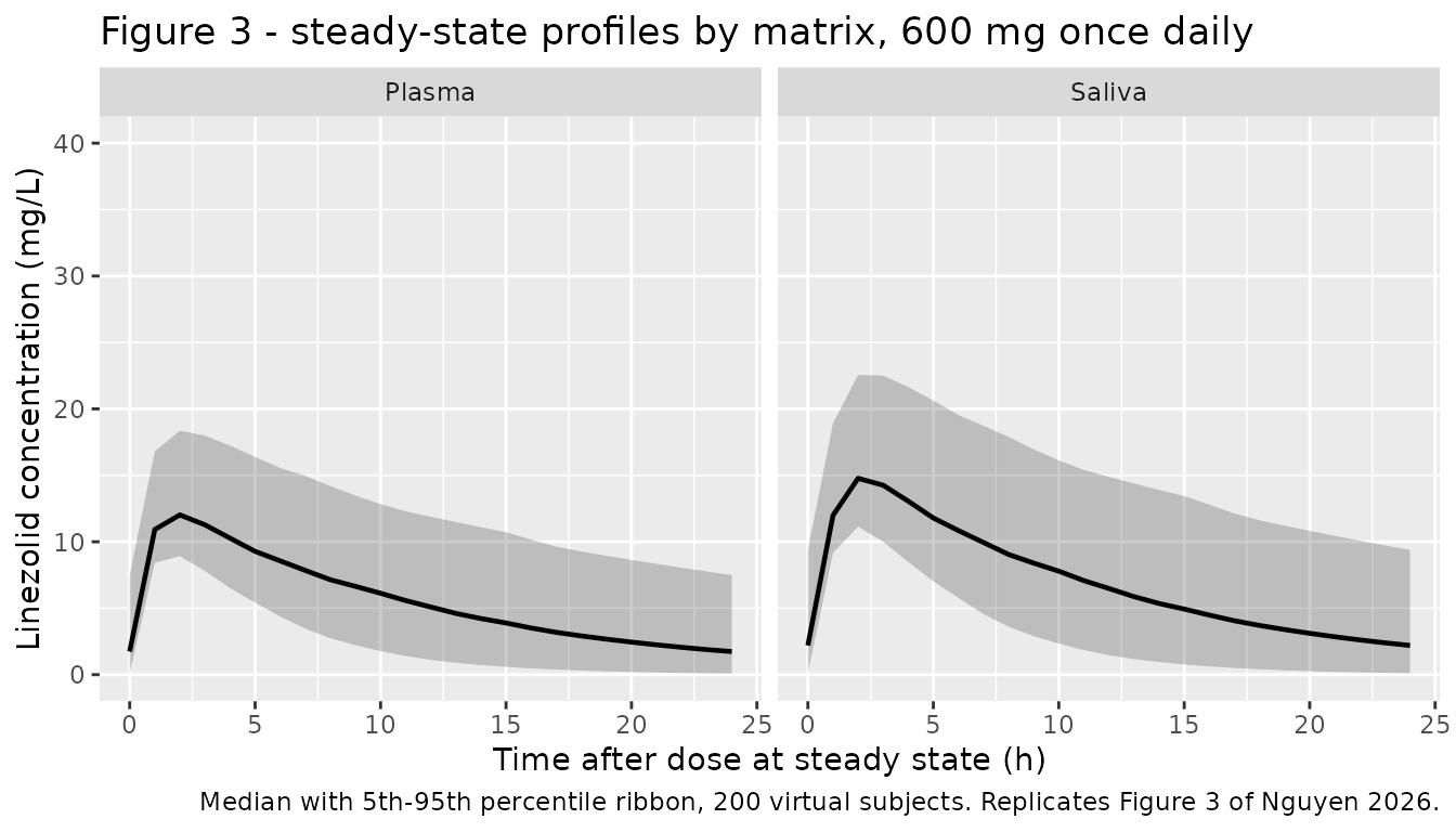
# Replicates Figure 3 of Nguyen 2026: steady-state concentration-time
# percentiles for plasma (left) and saliva (right). The paper's panels are
# limited to the 0-5 h observed sampling window on a shared 0-40 mg/L axis,
# with the saliva median sitting slightly above plasma; the full 24 h interval
# is shown here since the model is used to extrapolate to AUC(0-24).
sim |>
  filter(treatment == "600 mg q24h") |>
  select(id, tad, Plasma = Cc, Saliva = Csaliva) |>
  tidyr::pivot_longer(c(Plasma, Saliva), names_to = "matrix",
                      values_to = "conc") |>
  group_by(matrix, tad) |>
  summarise(
    Q05 = quantile(conc, 0.05),
    Q50 = quantile(conc, 0.50),
    Q95 = quantile(conc, 0.95),
    .groups = "drop"
  ) |>
  ggplot(aes(tad, Q50)) +
  geom_ribbon(aes(ymin = Q05, ymax = Q95), alpha = 0.25) +
  geom_line(linewidth = 0.8) +
  facet_wrap(~matrix) +
  coord_cartesian(ylim = c(0, 40)) +
  labs(
    x = "Time after dose at steady state (h)",
    y = "Linezolid concentration (mg/L)",
    title = "Figure 3 - steady-state profiles by matrix, 600 mg once daily",
    caption = paste(
      "Median with 5th-95th percentile ribbon, 200 virtual subjects.",
      "Replicates Figure 3 of Nguyen 2026."
    )
  )
The observed and reference sampling windows of Figure 4 and Tables 3-4 are outputs of Bayesian maximum-a-posteriori re-estimation over 18 limited-sampling designs, each with 300 Monte Carlo replicates per subject. Reproducing them requires refitting the model to simulated saliva data subject by subject, which is outside what a validation vignette does; those results are therefore not replicated here. What is checked is the model those simulations were run from – the structural identities above and the NCA table below.
PKNCA validation
sim_nca <- sim |>
  # Only `!is.na(Cc)`: adding `tad > 0` or `Cc > 0` would drop the time-zero
  # trough record that PKNCA anchors AUC(0-tau) on.
  filter(!is.na(Cc)) |>
  select(id, time = tad, Cc, treatment) |>
  arrange(treatment, id, time)

dose_df <- events |>
  filter(evid == 1, time == t_last) |>
  mutate(time = 0) |>
  select(id, time, amt, treatment)

conc_obj <- PKNCA::PKNCAconc(
  sim_nca, Cc ~ time | treatment + id,
  concu = "mg/L", timeu = "h"
)
dose_obj <- PKNCA::PKNCAdose(
  as.data.frame(dose_df), amt ~ time | treatment + id,
  doseu = "mg", route = "extravascular"
)

intervals <- data.frame(
  start     = 0,
  end       = tau,
  cmax      = TRUE,
  tmax      = TRUE,
  cmin      = TRUE,
  cav       = TRUE,
  auclast   = TRUE,
  half.life = TRUE
)

nca_res <- PKNCA::pk.nca(
  PKNCA::PKNCAdata(conc_obj, dose_obj, intervals = intervals)
)
# Second PKNCA block for the saliva output (multi-output model).
sal_nca <- sim |>
  filter(!is.na(Csaliva)) |>
  select(id, time = tad, Cc = Csaliva, treatment) |>
  arrange(treatment, id, time)

nca_sal <- PKNCA::pk.nca(
  PKNCA::PKNCAdata(
    PKNCA::PKNCAconc(sal_nca, Cc ~ time | treatment + id,
                     concu = "mg/L", timeu = "h"),
    dose_obj,
    intervals = intervals
  )
)
Comparison against published NCA
Nguyen 2026 Supplementary Table S6 reports steady-state NCA metrics computed from the model in NONMEM over 5100 virtual subjects, alongside an independent Bayesian re-analysis in Edsim++. The NONMEM column is the direct comparator for a simulation from this packaged model.
One caveat governs how to read the table. The paper’s simulations
“maintain the original study design”, i.e. each virtual subject carries
their real daily dose, which spanned 450-600 mg. AUC(0-24)
and Cmax are both directly proportional to dose, whereas
half-life and Tmax are dose-free. The 600 mg arm is therefore expected
to sit above the published AUC(0-24) and
Cmax by however much the study’s mean dose fell below 600
mg, and to match half-life and Tmax outright.
# Table S6, NONMEM (N = 5100) column. auclast over the 0-24 h steady-state
# interval is the paper's AUC(0-24).
published <- tibble::tribble(
  ~treatment,      ~auclast, ~half.life, ~cmax, ~tmax,
  "600 mg q24h",      131.5,       8.01,  11.2,  1.98
)

cmp <- nlmixr2lib::ncaComparisonTable(
  simulated     = nca_res,
  reference     = published,
  by            = "treatment",
  units         = c(auclast = "mg*h/L", cmax = "mg/L",
                    tmax = "h", half.life = "h"),
  tolerance_pct = 20
)

knitr::kable(
  cmp,
  caption = paste(
    "Simulated (600 mg once daily) vs Nguyen 2026 Table S6, NONMEM column.",
    "* differs from reference by >20%. The published values are for the",
    "study's mixed 450-600 mg daily doses; see the dose caveat above."
  ),
  align = c("l", "l", "r", "r", "r")
)| NCA parameter | treatment | Reference | Simulated | % diff |
|---|---|---|---|---|
| Cmax (mg/L) | 600 mg q24h | 11.2 | 12.3 | +9.7% |
| Tmax (h) | 600 mg q24h | 1.98 | 2 | +1.0% |
| AUClast (mg*h/L) | 600 mg q24h | 132 | 139 | +5.7% |
| t½ (h) | 600 mg q24h | 8.01 | 7.84 | -2.1% |
attr(cmp, "footnote")
#> NULL
ncaComparisonTable() aggregates the per-subject PKNCA
results with median(), which matters here and is worth
being explicit about. Every published metric in Table S6 is a
mean over 5100 subjects, but AUC(0-24) and
half-life are both proportional to 1/(CL/F) and therefore
log-normally distributed with a 47% CV, so their sample mean
over a 200-subject cohort has a standard error of about 3% and
drifts several percent between draws. Their sample
median is both the robust statistic and, for this
model, the exactly predictable one: the median of
Dose/(CL/F) over a log-normal CL/F is
Dose/(CL/F) at the typical value. Every assertion below is
therefore written on medians or on deterministic typical-value
quantities, never on a cohort mean.
The two dose-free metrics reproduce the published values closely, which is the sharper test of the structural model – they cannot be rescued by any dose assumption:
nca_tbl <- as.data.frame(nca_res$result) |>
  filter(treatment == "600 mg q24h") |>
  group_by(PPTESTCD) |>
  summarise(median = median(PPORRES), mean = mean(PPORRES), .groups = "drop")

# Guard against a silent zero-row lookup (a gate that cannot go red).
stopifnot(all(c("half.life", "tmax", "cmax", "auclast") %in% nca_tbl$PPTESTCD))
get_median <- function(code) {
  v <- nca_tbl$median[nca_tbl$PPTESTCD == code]
  if (length(v) != 1L) stop("no unique NCA row for '", code, "'")
  v
}

thalf_pct <- 100 * (get_median("half.life") / 8.01 - 1)
tmax_pct  <- 100 * (get_median("tmax") / 1.98 - 1)
c(half_life_pct_diff = thalf_pct, tmax_pct_diff = tmax_pct)
#> half_life_pct_diff      tmax_pct_diff
#>          -2.121251           1.010101

# The theoretical median half-life is ln2 * V/CL at the typical value, since
# neither V's weight term nor CL's eta shifts a median.
log(2) * 46.8 / 4.35
#> [1] 7.457308

# Bounds on a cohort MEDIAN. The sample median of a 47%-CV log-normal over 200
# subjects carries roughly a 4% standard error, so 12% is about 3 SE of
# headroom -- while a mis-transcribed clearance or volume moves ln2*V/CL by
# tens of percent and still goes red. Tmax is quantised to the paper's hourly
# grid, so any error in Ka moves it by a whole hour (>= 50%).
stopifnot(abs(thalf_pct) < 12)
stopifnot(abs(tmax_pct) < 12)
And the dose-proportional metrics are bracketed by the two arms, which is what the mixed-dose explanation predicts. The bracket is asserted on the deterministic typical-value exposures from the closed-form block above, so it carries no cohort-draw noise at all:
cohort_median <- as.data.frame(nca_res$result) |>
  filter(PPTESTCD %in% c("auclast", "cmax")) |>
  group_by(treatment, PPTESTCD) |>
  summarise(m = median(PPORRES), .groups = "drop") |>
  tidyr::pivot_wider(names_from = treatment, values_from = m)

typical <- cf_res |>
  select(treatment, auclast = auc_pl, cmax = cmax_pl) |>
  tidyr::pivot_longer(-treatment, names_to = "PPTESTCD",
                      values_to = "typical") |>
  tidyr::pivot_wider(names_from = treatment, values_from = typical)

bracket <- cohort_median |>
  left_join(typical, by = "PPTESTCD",
            suffix = c("_cohort_median", "_typical")) |>
  mutate(published = if_else(PPTESTCD == "auclast", 131.5, 11.2)) |>
  dplyr::rename(
    "NCA parameter"              = PPTESTCD,
    "450 mg typical"             = `450 mg q24h_typical`,
    "600 mg typical"             = `600 mg q24h_typical`,
    "450 mg cohort median"       = `450 mg q24h_cohort_median`,
    "600 mg cohort median"       = `600 mg q24h_cohort_median`,
    "Table S6 (450-600 mg mix)"  = published
  )

knitr::kable(
  bracket, digits = 2,
  caption = paste(
    "The published mixed-dose means fall between the 450 mg and 600 mg arms,",
    "as expected for quantities directly proportional to dose."
  )
)| NCA parameter | 450 mg cohort median | 600 mg cohort median | 600 mg typical | 450 mg typical | Table S6 (450-600 mg mix) |
|---|---|---|---|---|---|
| auclast | 102.49 | 139.05 | 137.93 | 103.45 | 131.5 |
| cmax | 9.39 | 12.29 | 12.05 | 9.04 | 11.2 |
# Deterministic bracket: Dose/(CL/F) at 450 and 600 mg must straddle the
# published mixed-dose mean. Goes red if CL/F is mis-transcribed in either
# direction (e.g. 5.5 L/h would put the 600 mg arm below 131.5).
tv <- function(arm, code) {
  v <- cf_res[[code]][cf_res$treatment == arm]
  if (length(v) != 1L) stop("no unique typical-value row for ", arm)
  v
}
stopifnot(tv("450 mg q24h", "auc_pl") < 131.5)
stopifnot(tv("600 mg q24h", "auc_pl") > 131.5)
stopifnot(tv("450 mg q24h", "cmax_pl") < 11.2)
stopifnot(tv("600 mg q24h", "cmax_pl") > 11.2)
The saliva NCA has no published comparator – Nguyen 2026 reports saliva exposure only through the saliva:plasma ratio already gated above – so it is reported for completeness rather than compared:
as.data.frame(nca_sal$result) |>
  filter(PPTESTCD %in% c("auclast", "cmax", "tmax", "cmin")) |>
  group_by(treatment, PPTESTCD) |>
  summarise(
    median = median(PPORRES),
    q05    = quantile(PPORRES, 0.05),
    q95    = quantile(PPORRES, 0.95),
    .groups = "drop"
  ) |>
  dplyr::rename(
    "Arm"           = treatment,
    "NCA parameter" = PPTESTCD,
    "Median"        = median,
    "5th pctile"    = q05,
    "95th pctile"   = q95
  ) |>
  knitr::kable(
    digits = 2,
    caption = "Simulated saliva NCA over the steady-state dosing interval."
)| Arm | NCA parameter | Median | 5th pctile | 95th pctile |
|---|---|---|---|---|
| 450 mg q24h | auclast | 128.53 | 60.65 | 265.55 |
| 450 mg q24h | cmax | 11.65 | 7.93 | 16.42 |
| 450 mg q24h | cmin | 1.50 | 0.11 | 6.03 |
| 450 mg q24h | tmax | 2.00 | 2.00 | 3.00 |
| 600 mg q24h | auclast | 174.03 | 83.28 | 351.16 |
| 600 mg q24h | cmax | 15.21 | 10.64 | 22.75 |
| 600 mg q24h | cmin | 2.20 | 0.20 | 8.36 |
| 600 mg q24h | tmax | 2.00 | 2.00 | 3.00 |
Exposure targets
Nguyen 2026 states an efficacy target of
fAUC(0-24)/MIC >= 125 with an assumed unbound fraction
of 87.2% and a surrogate MIC of 0.5 mg/L for M. tuberculosis,
and a toxicity threshold of total
AUC(0-24) > 283.6 mg*h/L (about a trough above 8.2
mg/L). Those thresholds translate into total-plasma
AUC(0-24) bounds and are shown here as an illustration of
how the model is used clinically. The paper reports no attainment table
for them, so this is not a published-value comparison and is not gated
against one.
fu        <- 0.872          # Nguyen 2026 Methods 2.4.2, from reference [34]
mic       <- 0.5            # mg/L, surrogate MIC, Methods 2.4.2
auc_eff   <- 125 * mic / fu # total-plasma AUC(0-24) meeting fAUC/MIC >= 125
auc_tox   <- 283.6          # mg*h/L, Introduction, from reference [11]
c(efficacy_threshold = auc_eff, toxicity_threshold = auc_tox)
#> efficacy_threshold toxicity_threshold
#>           71.67431          283.60000

as.data.frame(nca_res$result) |>
  filter(PPTESTCD == "auclast") |>
  group_by(treatment) |>
  summarise(
    `Median AUC(0-24)`   = median(PPORRES),
    `% above efficacy`   = 100 * mean(PPORRES >= auc_eff),
    `% above toxicity`   = 100 * mean(PPORRES > auc_tox),
    .groups = "drop"
  ) |>
  dplyr::rename("Arm" = treatment) |>
  knitr::kable(
    digits = 1,
    caption = paste(
      "Illustrative target attainment against the thresholds Nguyen 2026",
      "states. Not a published-value comparison."
    )
)| Arm | Median AUC(0-24) | % above efficacy | % above toxicity |
|---|---|---|---|
| 450 mg q24h | 102.5 | 73.5 | 0.0 |
| 600 mg q24h | 139.0 | 92.0 | 4.5 |
Assumptions and deviations
Reconstruction of the saliva ODE (structural, load-bearing)
Nguyen 2026 publishes its control stream in Supplementary Table S7,
but the table is headed “Example of NONMEM model code”
and is abridged: it declares $SUBROUTINE ADVAN13, the
general nonlinear solver, whose differential equations must be
written out in a $DES block – and no $DES
block is printed. The three saliva rate constants therefore had to be
assembled into an ODE, and the K23 / K32 /
K30 naming (borrowed from NONMEM’s general linear
ADVAN5/ADVAN7 subroutines, where those names do imply a
mass-balance matrix) suggests a reading that turns out to be wrong.
Two readings were solved in rxode2 and scored against the paper’s printed values:
-
Mass-balance exchange – central loses
kin_saliva * centraland regainskout_saliva * saliva. At steady stateA_saliva / A_central = 1.242, so loss through saliva iskel_saliva * 1.242 = 2.645per hour against a plasmakelof4.35 / 46.8 = 0.0929per hour: salivary elimination would be 28 times the plasma clearance. Solved, this gives a steady-state plasmaAUC(0-24)of 4.7mg*h/Land aCmaxof 2.8 mg/L. -
Driven (non-depleting) effect compartment – the
central equation carries neither term. Solved at the typical value, this
gives
AUC(0-24) = Dose/(CL/F) =137.9mg*h/LandCmax12.1 mg/L; on the paper’s own hourly grid the 200-subject cohort medians are 7.78 h for half-life and 2.0 h for Tmax.
Table S6 reports 131.5 mg*h/L, 11.2 mg/L, 8.01 h and
1.98 h. The mass-balance reading is out by roughly 28-fold on exposure
and 4-fold on Cmax; the driven reading matches the two
dose-free metrics to within 3% (-2.8% on half-life, +1.0% on Tmax) and
the two dose-proportional metrics to within 11% (+4.9% on
AUC(0-24), +10.3% on Cmax), with that residual
accounted for by the study’s 450-600 mg dose mix – the published means
fall inside the two-arm bracket above. Independently, this is exactly
what Figure 1’s caption says the compartment is: “The saliva
bio-compartment is a hypothetical effect compartment.” The driven form
is what the model file encodes. No printed parameter value was
altered to reach it – all seven structural estimates are used
exactly as published; only the unprinted $DES was
reconstructed.
Saliva concentration scaling
Table S7’s $ERROR block prints CP = A(2)/V
for plasma but CS = A(3) for saliva – i.e. a saliva
“concentration” equal to the saliva amount, an implied 1 L
scale. Taken literally, the steady-state saliva:plasma exposure ratio
becomes
V * kin_saliva / (kout_saliva + kel_saliva) = 46.8 * 1.242 = 58.1,
so saliva would run about 58 times plasma (roughly 650 mg/L against a
plasma Cmax of 11.2 mg/L) – outside the assay’s range and
contradicted by Figure 3, which plots both matrices on one shared 0-40
mg/L axis with the saliva median only slightly above plasma. Dividing by
vc gives 1.2418, matching the paper’s own independently
reported 1.27 (95% CI 1.09-1.44) to 2%. The model encodes
Csaliva <- saliva / vc. Ratified by the maintainers on
2026-09-02.
Other assumptions
-
Weight distribution. Table 1 reports weight as a
median and IQR only, with no full range. The virtual cohort draws weight
log-normally with median 50 kg and a log-scale SD chosen so the
simulated IQR reproduces 45-56 kg. The weight exponent on
V/Fwas fitted over that narrow, lean range (median BMI 19.1 kg/m^2) and its 95% CI (0.62-1.46) spans 1, so it extrapolates poorly to heavier populations. - Dose levels. The study’s per-subject daily doses are not published, only the median (600 mg) and range (450-600 mg). The vignette simulates the two endpoints of that range as separate arms rather than guessing a mix.
-
No IIV on five parameters.
V/F,Ka,F,Kabs,KreabsandKelcarry no between-subject variability, because Table S7 fixes all six$OMEGAelements to zero and Results 3.2 explains that saliva-specific rate-constant IIV had shrinkage above 55%. They are omitted fromini()rather than written as~ fixed(0), which would make OMEGA singular and break rxode2’s Cholesky sampler. -
KaandFare fixed, not estimated. Both are wrapped infixed()so a user re-fitting the model inherits the authors’ identifiability constraint rather than silently estimating a parameter the design cannot support. The reported parameters are apparent (CL/F,V/F) as a consequence. -
Sex is absent by design. With 14 male and 3 female
subjects the authors did not test sex as a covariate, so the model
carries no sex term. This is recorded in
population$notes, not as a screened-and-rejected covariate. -
Screened covariates. Age, creatinine clearance,
serum creatinine, ALT, AST and platelet count were screened and not
retained (Results 3.2, Supplementary Figure S8). They appear in the
model file’s
covariatesDataExcludedmetadata for provenance and are deliberately absent frommodel(). - Bayesian limited-sampling results are not replicated. Tables 3 and 4 and Figure 4 report maximum-a-posteriori re-estimation across 18 sampling designs; see the note under Replicate published figures.
-
No non-paper-derived parameter values. Every
ini()entry comes from Nguyen 2026 Table 2 or the Table S7 control stream. Nothing was digitised from a figure, supplied by correspondence, or carried from an upstream model.