Eflornithine (Jansson 2008)
Source:vignettes/articles/Jansson_2008_eflornithine.Rmd
Jansson_2008_eflornithine.RmdModel and source
- Citation: Jansson R, Malm M, Roth C, Ashton M. Enantioselective and nonlinear intestinal absorption of eflornithine in the rat. Antimicrob Agents Chemother. 2008;52(8):2842-2848.
- Article: https://doi.org/10.1128/aac.00050-08
- Description: stereoselective two-enantiomer popPK of racemic eflornithine in male Sprague-Dawley rats after single oral or IV doses. Each enantiomer (L = active, D) carries its own 2-compartment disposition; oral absorption is modeled with a shared Savic 2007 transit-compartment chain feeding per-enantiomer depots that drain to central via saturable Michaelis-Menten kinetics. Bioavailability differs between L and D and shifts upward at the highest oral dose (3000 mg/kg) via a categorical covariate.
Population
Sixty-nine male Sprague-Dawley rats weighing 260-320 g (typical 290 g) were dosed once with racemic eflornithine hydrochloride. Forty-one rats received oral doses by gavage at 750, 1500, 2000, or 3000 mg/kg (10 mL/kg solution) for chiral assay and an additional 16 rats received the same dose levels for racemic assay. Twelve rats received IV doses at 375 or 1000 mg/kg via the jugular vein catheter (3-min infusion, modeled as a bolus). Source: Jansson 2008 Table 1.
The same metadata is available programmatically via
rxode2::rxode(readModelDb("Jansson_2008_eflornithine_rat"))$population.
Source trace
The per-parameter origin is recorded as an in-file comment next to
each ini() entry in
inst/modeldb/specificDrugs/Jansson_2008_eflornithine_rat.R.
The table below collects them.
| Parameter | Value (mg / h / L for a 290 g rat) | Paper value | Source location |
|---|---|---|---|
lcl_l |
log(0.2523) L/h | CL_L = 14.5 mL/min/kg | Table 2 |
lcl_d |
log(0.2192) L/h | CL_D = 12.6 mL/min/kg | Table 2 |
lvc_l |
log(0.1172) L | Vc_L = 0.404 L/kg | Table 2 |
lvc_d |
log(0.1163) L | Vc_D = 0.401 L/kg | Table 2 |
lq |
log(0.02088) L/h | Q = 1.2 mL/min/kg (shared) | Table 2 |
lvp |
log(0.1293) L | Vp = 0.446 L/kg (shared) | Table 2 |
lmtt |
log(1.467) h | MTT = 88 min (shared) | Table 3 |
lnn |
log(1.424) | n = 1.424 transit compartments (shared) | Table 3 |
ltmax_abs_l |
log(35.18) mg/h | Tmax_L = 11.1 umol/min/kg | Table 3 |
ltmax_abs_d |
log(45.95) mg/h | Tmax_D = 14.5 umol/min/kg | Table 3 |
lkt_abs_l |
log(82.41) mg | Kt_L = 1560 umol/kg | Table 3 |
lkt_abs_d |
log(41.42) mg | Kt_D = 784 umol/kg | Table 3 |
lfdepot_l |
log(0.41) | F_L (750-2000 mg/kg) = 41% | Table 3 |
lfdepot_d |
log(0.623) | F_D (750-2000 mg/kg) = 62.3% | Table 3 |
e_dose_high_efl_fdepot_l |
0.1463 | F_L (3000) = 47% (+14.6% vs reference) | Table 3 + Results |
e_dose_high_efl_fdepot_d |
0.3275 | F_D (3000) = 82.7% (+32.8% vs reference) | Table 3 + Results |
etalcl_l |
0.02197 | IIV CL_L = 14.9% CV | Table 2 |
etalcl_d |
0.03263 | IIV CL_D = 18.2% CV | Table 2 |
etalmtt |
0.1349 | IIV MTT = 38% CV (shared) | Table 3 |
etalfdepot |
0.00995 | IIV F = 10% CV (shared) | Table 3 |
propSd_l/d/rac |
0.277 | Oral residual sigma = 27.7% CV (proportional) | Table 3 + Methods |
| Transit chain (Savic 2007 analytical) | n/a | “transit model followed by a Michaelis-Menten function” | Fig 1 + Results paragraph |
| Saturable absorption rate | n/a | dA_central/dt receives Tmax*A_depot/(Kt+A_depot) | Fig 1 + Results paragraph |
| 2-compartment IV disposition | n/a | “biphasic” IV profile | Methods + Results + Fig 2 |
Virtual cohort
Original observed data are not publicly available. Below we simulate the typical-value plasma profiles for each dose group reported in the paper. A virtual cohort with between-subject variability is constructed at the end of the vignette for an illustrative VPC.
The dose record convention for this model: each oral administration
generates two dose rows (one to depot_l
and one to depot_d, each with amt = 50% of the
total racemic dose) so each enantiomer’s transit chain reads its own
podo() / tad(). IV doses follow the same 50/50
split into central_l and central_d. This is
dictated by rxode2’s requirement that the dose target compartment be the
same compartment whose d/dt() carries the
transit() call.
RAT_WT_KG <- 0.290  # typical Sprague-Dawley body weight in the Jansson 2008 cohort
EFL_MW    <- 182.17 # eflornithine molar mass (g/mol), used for uM <-> ug/mL conversions

# Dose levels (mg/kg racemic; Table 1) and matched high-dose indicators.
oral_doses <- tibble(
  dose_mgkg     = c(750, 1500, 2000, 3000),
  DOSE_HIGH_EFL = c(0,   0,    0,    1)
)

iv_doses <- tibble(
  dose_mgkg     = c(375, 1000),
  DOSE_HIGH_EFL = c(0,   0)
)

# Build a single-subject event table for an oral or IV regimen.
# id_offset shifts subject IDs so multiple cohorts can be bind_rows()-ed.
make_oral_events <- function(dose_mgkg, DOSE_HIGH_EFL, obs_times,
                             id = 1L, wt_kg = RAT_WT_KG) {
  amt_total <- dose_mgkg * wt_kg          # total racemic dose (mg)
  amt_half  <- amt_total * 0.5            # 50/50 enantiomer split
  bind_rows(
    tibble(id = id, time = 0, evid = 1L, cmt = "depot_l",  amt = amt_half),
    tibble(id = id, time = 0, evid = 1L, cmt = "depot_d",  amt = amt_half),
    tibble(id = id, time = obs_times, evid = 0L,
           cmt = "Cc_l", amt = NA_real_)
  ) |> mutate(DOSE_HIGH_EFL = DOSE_HIGH_EFL,
              dose_mgkg     = dose_mgkg,
              regimen       = sprintf("Oral %d mg/kg", dose_mgkg))
}

make_iv_events <- function(dose_mgkg, DOSE_HIGH_EFL, obs_times,
                           id = 1L, wt_kg = RAT_WT_KG) {
  amt_total <- dose_mgkg * wt_kg
  amt_half  <- amt_total * 0.5
  bind_rows(
    tibble(id = id, time = 0, evid = 1L, cmt = "central_l", amt = amt_half),
    tibble(id = id, time = 0, evid = 1L, cmt = "central_d", amt = amt_half),
    tibble(id = id, time = obs_times, evid = 0L,
           cmt = "Cc_l", amt = NA_real_)
  ) |> mutate(DOSE_HIGH_EFL = DOSE_HIGH_EFL,
              dose_mgkg     = dose_mgkg,
              regimen       = sprintf("IV %d mg/kg", dose_mgkg))
}

oral_obs <- c(0.05, seq(0.5, 30, by = 0.5))
iv_obs   <- c(0.083, 0.25, seq(0.5, 18, by = 0.5))
Simulation
Typical-value profiles (random effects zeroed) for each oral and IV dose level reported in the paper:
mod         <- readModelDb("Jansson_2008_eflornithine_rat")
mod_typical <- rxode2::zeroRe(mod)
#> ℹ parameter labels from comments will be replaced by 'label()'

sim_oral <- purrr::map2_dfr(oral_doses$dose_mgkg, oral_doses$DOSE_HIGH_EFL,
  function(d, hi) {
    ev <- make_oral_events(d, hi, oral_obs)
    rxode2::rxSolve(mod_typical, events = ev,
                    keep = c("dose_mgkg", "regimen", "DOSE_HIGH_EFL")) |>
      as_tibble() |>
      mutate(id = 1L)
  }
)
#> ℹ omega/sigma items treated as zero: 'etalcl_l', 'etalcl_d', 'etalmtt', 'etalfdepot'
#> ℹ omega/sigma items treated as zero: 'etalcl_l', 'etalcl_d', 'etalmtt', 'etalfdepot'
#> ℹ omega/sigma items treated as zero: 'etalcl_l', 'etalcl_d', 'etalmtt', 'etalfdepot'
#> ℹ omega/sigma items treated as zero: 'etalcl_l', 'etalcl_d', 'etalmtt', 'etalfdepot'

sim_iv <- purrr::map2_dfr(iv_doses$dose_mgkg, iv_doses$DOSE_HIGH_EFL,
  function(d, hi) {
    ev <- make_iv_events(d, hi, iv_obs)
    rxode2::rxSolve(mod_typical, events = ev,
                    keep = c("dose_mgkg", "regimen", "DOSE_HIGH_EFL")) |>
      as_tibble() |>
      mutate(id = 1L)
  }
)
#> ℹ omega/sigma items treated as zero: 'etalcl_l', 'etalcl_d', 'etalmtt', 'etalfdepot'
#> ℹ omega/sigma items treated as zero: 'etalcl_l', 'etalcl_d', 'etalmtt', 'etalfdepot'
Replicate published figures
Concentrations on the plots are converted to micromolar (the paper’s
units) via Cc [uM] = Cc [ug/mL] * 1000 / MW.
# Replicates Figure 2 of Jansson 2008: IV plasma profile for L, D, and racemic
# eflornithine after 375 or 1000 mg/kg racemic dose. Concentrations in uM.
sim_iv |>
  pivot_longer(c(Cc_l, Cc_d, Cc_rac), names_to = "analyte", values_to = "Cc_ugmL") |>
  mutate(
    Cc_uM   = Cc_ugmL * 1000 / EFL_MW,
    analyte = factor(analyte,
                     levels = c("Cc_l", "Cc_d", "Cc_rac"),
                     labels = c("L-eflornithine", "D-eflornithine", "Racemic"))
  ) |>
  filter(time > 0, Cc_uM > 5) |>
  ggplot(aes(time, Cc_uM, color = factor(dose_mgkg), linetype = analyte)) +
  geom_line() +
  scale_y_log10() +
  facet_wrap(~ analyte) +
  labs(x = "Time (h)", y = "Plasma concentration (uM)",
       color = "IV dose (mg/kg)", linetype = "Analyte",
       title = "Figure 2 (typical-value) - IV eflornithine in rat",
       caption = "Replicates Figure 2 of Jansson 2008.")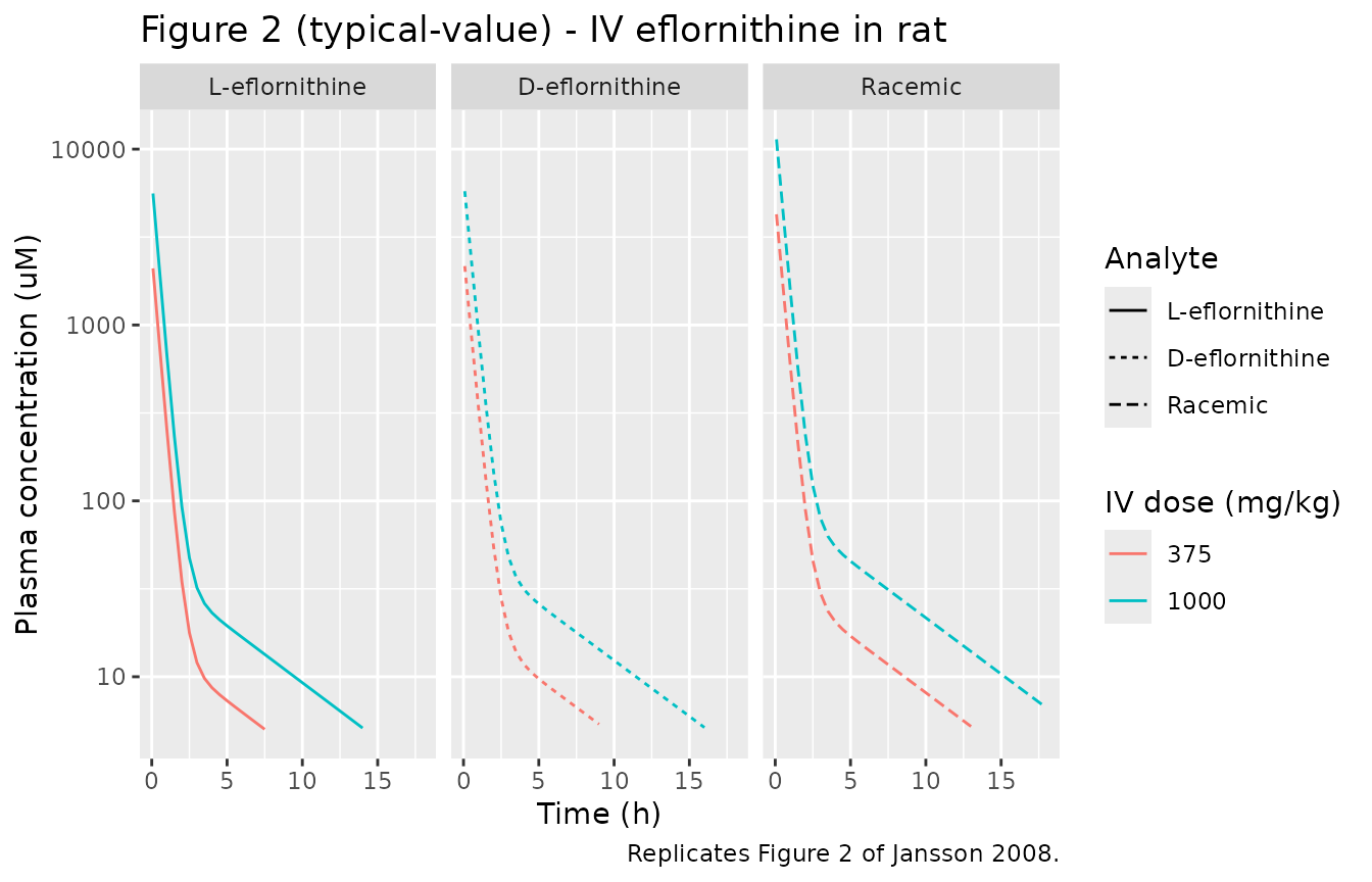
# Replicates Figure 4 of Jansson 2008: oral plasma profile for L, D, and racemic
# eflornithine after 750, 1500, 2000, or 3000 mg/kg racemic doses. Tmax shifts
# from ~1.5 h at 750 mg/kg to ~6 h at 3000 mg/kg via the saturable absorption.
sim_oral |>
  pivot_longer(c(Cc_l, Cc_d, Cc_rac), names_to = "analyte", values_to = "Cc_ugmL") |>
  mutate(
    Cc_uM   = Cc_ugmL * 1000 / EFL_MW,
    analyte = factor(analyte,
                     levels = c("Cc_l", "Cc_d", "Cc_rac"),
                     labels = c("L-eflornithine", "D-eflornithine", "Racemic"))
  ) |>
  filter(Cc_uM > 5) |>
  ggplot(aes(time, Cc_uM, color = factor(dose_mgkg))) +
  geom_line() +
  scale_y_log10() +
  facet_wrap(~ analyte) +
  labs(x = "Time (h)", y = "Plasma concentration (uM)",
       color = "Oral dose (mg/kg)",
       title = "Figure 4 (typical-value) - Oral eflornithine in rat",
       caption = "Replicates Figure 4 of Jansson 2008. Tmax shifts upward with dose; F_L stays at 41-47% while F_D jumps to 83% at the highest dose.")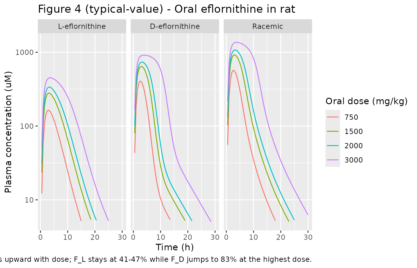
PKNCA validation
We compute Cmax, Tmax, AUC0-inf, and apparent half-life for each enantiomer and the racemic sum after each oral dose. The paper does not tabulate NCA values directly, but we use them to verify three model features mentioned in the Results: (i) Tmax shifts upward with dose, (ii) racemic-eflornithine bioavailability rises with dose (F_rac = (F_L + F_D)/2 = 51.6% at the lower doses and 64.9% at 3000 mg/kg), and (iii) the model’s saturable absorption produces non-proportional dose-AUC scaling.
# Reshape oral typical-value simulation into a long PKNCA-friendly form.
sim_oral_long <- sim_oral |>
  pivot_longer(c(Cc_l, Cc_d, Cc_rac),
               names_to = "analyte", values_to = "Cc_ugmL") |>
  filter(!is.na(Cc_ugmL), time > 0) |>
  mutate(amt_dose_l   = dose_mgkg * RAT_WT_KG * 0.5,
         amt_dose_rac = dose_mgkg * RAT_WT_KG) |>
  select(id, regimen, dose_mgkg, analyte, time, Cc_ugmL,
         amt_dose_l, amt_dose_rac)

run_pknca_one <- function(df, dose_amt_col) {
  conc_df <- df |>
    mutate(uid = paste(regimen, id)) |>
    select(uid, time, Cc = Cc_ugmL, regimen)
  dose_df <- df |>
    distinct(uid = paste(regimen, id), regimen,
             amt = .data[[dose_amt_col]]) |>
    mutate(time = 0)
  cobj <- PKNCA::PKNCAconc(conc_df, Cc ~ time | regimen + uid)
  dobj <- PKNCA::PKNCAdose(dose_df, amt ~ time | regimen + uid)
  intervals <- data.frame(start = 0, end = Inf,
                          cmax = TRUE, tmax = TRUE,
                          aucinf.obs = TRUE, half.life = TRUE)
  PKNCA::pk.nca(PKNCA::PKNCAdata(cobj, dobj, intervals = intervals))
}

nca_l <- sim_oral_long |>
  filter(analyte == "Cc_l") |>
  run_pknca_one("amt_dose_l")
#> Warning: Requesting an AUC range starting (0) before the first measurement (0.05) is not allowed
#> Requesting an AUC range starting (0) before the first measurement (0.05) is not allowed
#> Requesting an AUC range starting (0) before the first measurement (0.05) is not allowed
#> Requesting an AUC range starting (0) before the first measurement (0.05) is not allowed

nca_d <- sim_oral_long |>
  filter(analyte == "Cc_d") |>
  run_pknca_one("amt_dose_l")    # D dose = same 50% split
#> Warning: Requesting an AUC range starting (0) before the first measurement (0.05) is not allowed
#> Requesting an AUC range starting (0) before the first measurement (0.05) is not allowed
#> Requesting an AUC range starting (0) before the first measurement (0.05) is not allowed
#> Requesting an AUC range starting (0) before the first measurement (0.05) is not allowed

nca_rac <- sim_oral_long |>
  filter(analyte == "Cc_rac") |>
  run_pknca_one("amt_dose_rac")  # racemic dose denominator
#> Warning: Requesting an AUC range starting (0) before the first measurement (0.05) is not allowed
#> Requesting an AUC range starting (0) before the first measurement (0.05) is not allowed
#> Requesting an AUC range starting (0) before the first measurement (0.05) is not allowed
#> Requesting an AUC range starting (0) before the first measurement (0.05) is not allowed

summarise_nca <- function(nca_obj, label) {
  as.data.frame(nca_obj$result) |>
    filter(PPTESTCD %in% c("cmax", "tmax", "aucinf.obs", "half.life")) |>
    mutate(analyte = label)
}

nca_table <- bind_rows(
  summarise_nca(nca_l,   "L-eflornithine"),
  summarise_nca(nca_d,   "D-eflornithine"),
  summarise_nca(nca_rac, "Racemic")
) |>
  select(analyte, regimen, PPTESTCD, PPORRES) |>
  pivot_wider(names_from = PPTESTCD, values_from = PPORRES)

knitr::kable(nca_table,
             caption = "Simulated NCA parameters by oral dose group (typical value). Cmax in ug/mL; AUC in ug*h/mL; Tmax and half-life in h.",
digits = 3)| analyte | regimen | cmax | tmax | half.life | aucinf.obs |
|---|---|---|---|---|---|
| L-eflornithine | Oral 1500 mg/kg | 50.961 | 3.0 | 4.411 | NA |
| L-eflornithine | Oral 2000 mg/kg | 61.377 | 3.0 | 4.366 | NA |
| L-eflornithine | Oral 3000 mg/kg | 82.149 | 3.5 | 4.189 | NA |
| L-eflornithine | Oral 750 mg/kg | 29.862 | 3.0 | 4.457 | NA |
| D-eflornithine | Oral 1500 mg/kg | 116.946 | 3.0 | 4.706 | NA |
| D-eflornithine | Oral 2000 mg/kg | 134.200 | 3.0 | 4.706 | NA |
| D-eflornithine | Oral 3000 mg/kg | 166.412 | 4.0 | 4.707 | NA |
| D-eflornithine | Oral 750 mg/kg | 74.215 | 2.5 | 4.711 | NA |
| Racemic | Oral 1500 mg/kg | 167.908 | 3.0 | 4.547 | NA |
| Racemic | Oral 2000 mg/kg | 195.578 | 3.0 | 4.518 | NA |
| Racemic | Oral 3000 mg/kg | 248.152 | 4.0 | 4.448 | NA |
| Racemic | Oral 750 mg/kg | 103.445 | 2.5 | 4.564 | NA |
The Tmax column should rise monotonically with dose (a structural prediction of the saturable absorption from the depot - higher amounts saturate the rate and prolong the time-to-peak). The AUC column should rise less than proportionally with dose at the lower dose levels (saturation lowers F_eff) and then jump at 3000 mg/kg via the categorical F adjustment.
Optional VPC with between-subject variability
N_PER_GROUP <- 12L
oral_obs_vpc <- seq(0, 24, by = 1)

vpc_events <- purrr::pmap_dfr(oral_doses,
  function(dose_mgkg, DOSE_HIGH_EFL) {
    purrr::map_dfr(seq_len(N_PER_GROUP),
      function(k) {
        id <- as.integer(dose_mgkg * 100L + k)  # disjoint IDs across groups
        make_oral_events(dose_mgkg, DOSE_HIGH_EFL, oral_obs_vpc, id = id)
      })
  })

set.seed(459L)
vpc_sim <- rxode2::rxSolve(mod, events = vpc_events,
                           keep = c("dose_mgkg", "regimen", "DOSE_HIGH_EFL")) |>
  as_tibble()
#> ℹ parameter labels from comments will be replaced by 'label()'

vpc_sim |>
  filter(time > 0, Cc_rac > 0) |>
  mutate(Cc_uM = Cc_rac * 1000 / EFL_MW) |>
  group_by(regimen, time) |>
  summarise(Q05 = quantile(Cc_uM, 0.05),
            Q50 = quantile(Cc_uM, 0.50),
            Q95 = quantile(Cc_uM, 0.95),
            .groups = "drop") |>
  ggplot(aes(time, Q50, color = regimen, fill = regimen)) +
  geom_ribbon(aes(ymin = Q05, ymax = Q95), alpha = 0.18, color = NA) +
  geom_line() +
  scale_y_log10() +
  labs(x = "Time (h)", y = "Racemic plasma concentration (uM)",
       title = sprintf("VPC of racemic eflornithine after oral dosing (n=%d per group)", N_PER_GROUP),
       caption = "Median and 5th-95th percentile envelope from rxSolve with between-subject variability.")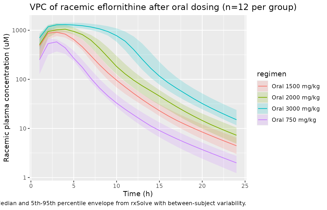
Assumptions and deviations
-
Residual error documentation conflict in the
source. Jansson 2008 Methods text says “Random residual
variability was modeled as proportional to the observed concentrations”
and Table 3’s sigma column carries the header “(% coefficient of
variation)” - both consistent with a proportional residual on the linear
scale. Table 3 footnote ‘a’ mislabels sigma as “additive residual
error”, which is internally inconsistent. The model encodes proportional
residual error (
prop(propSd_l/d/rac)). -
IV vs oral residual. The paper estimated separate
proportional residuals for the IV fit (sigma = 19.9% CV, Table 2) and
the oral fit (sigma = 27.7% CV, Table 3). For multi-output simulation
simplicity, this model uses 27.7% CV for all three plasma outputs (L, D,
racemic). The IV residual is slightly overestimated as a consequence.
Downstream users running IV-only simulations may override
propSd_l/d/racto 0.199 to recover the paper’s IV residual exactly. - Body weight reference (290 g). Per-kg parameter values from Tables 2 and 3 are converted to absolute units (L, L/h, mg, mg/h) using the midpoint study weight 0.290 kg. The cohort range was 260-320 g; users simulating individual rats outside that midpoint may need to scale linearly (volumes) or via allometric exponent 0.75 (clearances) - the package’s standard allometric scaffolding is not built in here because the within-cohort weight range is narrow.
-
Dose record convention. Each racemic administration
creates two dose rows (50% to depot_l / central_l for L, 50% to depot_d
/ central_d for D), reflecting the 50:50 molecular composition of
racemic eflornithine. rxode2’s
transit()function requires the dose target compartment to coincide with the d/dt() call site, so a single shared “depot” compartment is not used; instead each enantiomer carries its own depot and central. Users feeding the model their own data must therefore split each racemic dose into the two halves before passing it torxSolve(). -
Shared transit-chain IIV (etalmtt) acts on both enantiomers
via the single shared
mttparameter. Shared bioavailability IIV (etalfdepot) is applied as one random effect that scales bothfdepot_landfdepot_dsimultaneously (perfectly correlated between enantiomers). This matches the paper’s statement that “Interindividual variability values for mean transit time and bioavailability could not be estimated separately for D- and L-eflornithine and were therefore assumed to be identical.” -
High-dose categorical effect on F. Bioavailability
rises at the 3000 mg/kg oral dose level via a binary indicator
(
DOSE_HIGH_EFL = 1). The paper explicitly states that linear or power dose-F relationships did not improve the fit, so the categorical encoding is the published model form. Users simulating intermediate dose levels (>2000 and <3000 mg/kg) should set the indicator according to the paper’s threshold; the model does not interpolate. -
Original NONMEM control stream not on disk. The
Savic 2007 transit-chain Stirling approximation cited by the paper is
the analytical input form built into rxode2’s
transit()function, so no Stirling code is required in the model file.