Intra-CSF small molecules, LeiCNS-PK3.1 rat CNS PBPK (Hirasawa 2022)
Source:vignettes/articles/Hirasawa_2022_leicns_pk31_csf_flow.Rmd
Hirasawa_2022_leicns_pk31_csf_flow.RmdModel and source
- Citation: Hirasawa M, de Lange ECM. Revisiting Cerebrospinal Fluid Flow Direction and Rate in Physiologically Based Pharmacokinetic Model. Pharmaceutics. 2022;14(9):1764. doi:[10.3390/pharmaceutics14091764](https://doi.org/10.3390/pharmaceutics14091764).
- Upstream framework: Saleh MAA, Bloemberg JM, Elassaiss-Schaap J, de
Lange ECM. J Pharmacokinet Pharmacodyn. 2021;48(5):725-741. doi:[10.1007/s10928-021-09768-7](https://doi.org/10.1007/s10928-021-09768-7) (reference
[6] of the 2022 paper). Its Supplementary table 2 supplies the rat CNS
physiology and its Supplementary equations supply
Daq,P0,QpandQt.
Hirasawa 2022 revisits the cerebrospinal-fluid (CSF) part of the LeiCNS-PK3.0 CNS PBPK model. LeiCNS-PK3.0 moves drug through the CSF by one unidirectional, constant flow (2.2 uL/min in the rat) from the lateral ventricles (LV) to the third and fourth ventricles (TFV), cisterna magna (CM) and subarachnoid space (SAS). That model over-predicts the elimination from CM of seven of ten small molecules given into the CSF. The new LeiCNS-PK3.1 model (Figure 1B) has:
-
bidirectional, site-dependent CSF movement:
downward and upward rates between LV, TFV and CM
(
venQCSF,D,venQCSF,U) and between CM and SAS (cisQCSF,D,cisQCSF,U), with one up/down ratio; - a drug-specific transfer clearance from SAS to
plasma (
sasQCSF); - a choroid-plexus microvessel compartment (CPMV), separated from the whole-brain microvessels, which feeds both blood-CSF barriers (BCSFB);
- a correction factor on paracellular permeability
(
CFPPA).
The three drug-independent CSF parameters were estimated from
[3H]sucrose (ICV) and [14C]sucrose (intracisternal) data. They were then
fixed, and sasQCSF and CFPPA were estimated
for nine further molecules (Table 2). For three molecules the authors
also explored structural extensions (Supplementary Figures S2 and
S3).
Fifteen model files are packaged, one per parameterisation:
models <- tibble::tribble(
  ~model, ~molecule, ~role,
  "Hirasawa_2022_sucrose_rat_pbpk", "sucrose", "CSF parameters estimated (Table 2)",
  "Hirasawa_2022_inulin_rat_pbpk", "inulin", "Table 2",
  "Hirasawa_2022_morphine6Glucuronide_rat_pbpk", "morphine-6-glucuronide", "Table 2",
  "Hirasawa_2022_morphine_rat_pbpk", "morphine", "Table 2",
  "Hirasawa_2022_atenolol_rat_pbpk", "atenolol", "Table 2; van Bree 1989 plasma model",
  "Hirasawa_2022_atenolol_microdialysis_rat_pbpk", "atenolol", "Table 2; de Lange 1994 data, Saleh 2021 plasma model",
  "Hirasawa_2022_acetaminophen_rat_pbpk", "acetaminophen", "Table 2; van Bree 1989 plasma model",
  "Hirasawa_2022_acetaminophen_microdialysis_rat_pbpk", "acetaminophen", "Table 2; de Lange 1994 plasma model",
  "Hirasawa_2022_antipyrine_rat_pbpk", "antipyrine", "Table 2",
  "Hirasawa_2022_cefodizime_rat_pbpk", "cefodizime", "Table 2",
  "Hirasawa_2022_guanidinosuccinicAcid_rat_pbpk", "guanidinosuccinic acid", "Table 2",
  "Hirasawa_2022_ziconotide_rat_pbpk", "ziconotide", "Table 2",
  "Hirasawa_2022_morphine_bsc_rat_pbpk", "morphine", "Figure S2: + brain/spinal-cord surface compartment",
  "Hirasawa_2022_acetaminophen_periventricular_rat_pbpk", "acetaminophen", "Figure S3: + periventricular clearance",
  "Hirasawa_2022_antipyrine_periventricular_rat_pbpk", "antipyrine", "Figure S3: + periventricular clearance"
)
knitr::kable(models)| model | molecule | role |
|---|---|---|
| Hirasawa_2022_sucrose_rat_pbpk | sucrose | CSF parameters estimated (Table 2) |
| Hirasawa_2022_inulin_rat_pbpk | inulin | Table 2 |
| Hirasawa_2022_morphine6Glucuronide_rat_pbpk | morphine-6-glucuronide | Table 2 |
| Hirasawa_2022_morphine_rat_pbpk | morphine | Table 2 |
| Hirasawa_2022_atenolol_rat_pbpk | atenolol | Table 2; van Bree 1989 plasma model |
| Hirasawa_2022_atenolol_microdialysis_rat_pbpk | atenolol | Table 2; de Lange 1994 data, Saleh 2021 plasma model |
| Hirasawa_2022_acetaminophen_rat_pbpk | acetaminophen | Table 2; van Bree 1989 plasma model |
| Hirasawa_2022_acetaminophen_microdialysis_rat_pbpk | acetaminophen | Table 2; de Lange 1994 plasma model |
| Hirasawa_2022_antipyrine_rat_pbpk | antipyrine | Table 2 |
| Hirasawa_2022_cefodizime_rat_pbpk | cefodizime | Table 2 |
| Hirasawa_2022_guanidinosuccinicAcid_rat_pbpk | guanidinosuccinic acid | Table 2 |
| Hirasawa_2022_ziconotide_rat_pbpk | ziconotide | Table 2 |
| Hirasawa_2022_morphine_bsc_rat_pbpk | morphine | Figure S2: + brain/spinal-cord surface compartment |
| Hirasawa_2022_acetaminophen_periventricular_rat_pbpk | acetaminophen | Figure S3: + periventricular clearance |
| Hirasawa_2022_antipyrine_periventricular_rat_pbpk | antipyrine | Figure S3: + periventricular clearance |
Atenolol and acetaminophen each have two files because the paper uses two plasma PK models for them (Supplementary Table S1). One goes with the van Bree 1989 CSF data, to which Table 2 was fitted (Figure 4C,E); the other goes with the de Lange 1994 microdialysis data (Figure 4D,F). The CNS parameters are the same in both.
CNS structure
plasma <-(Q_CBF)-> brain_vascular <-(BBB)-> brain_ecf <-> brain_cell_membrane <-> brain_icf <-> brain_lysosome
plasma <-(Q_CPBF)-> brain_choroid_plexus_vascular <-(BCSFB)-> brain_csf_lv, brain_csf_tfv
brain_ecf --(Q_ECF)--> brain_csf_lv <-(venQ D/U)-> brain_csf_tfv <-(venQ D/U)-> brain_csf_cm <-(cisQ D/U)-> brain_csf_sas --(sasQCSF)--> plasma
All concentrations are unbound. The plasma model is the empirical
unbound model of Supplementary Table S1. It is mass-balanced with the
CNS, which is what lets drug dosed into the CSF reach plasma. Neutral
drug crosses a barrier by both the paracellular and the transcellular
route; charged drug only by the paracellular route. Asymmetry factors
(AF) carry active transport and are back-solved from the reported
Kp,uu values (Section 2.9; Supplementary Equations).
Population
All data are literature group means from healthy rats, digitised by the authors (Table 1). No original animals were studied. Rats are taken as 250 g (Section 2.5) when per-kg doses are converted. Doses into the CSF are split across the CSF compartments by the dosing-volume assumptions of Supplementary Table S3, and are given as instantaneous boluses (Section 2.5). Subject counts are those of the cited source studies and are not restated in the paper.
Source trace
trace_tab <- tibble::tribble(
  ~Quantity, ~`Source location`,
  "venQCSF,D 0.251, cisQCSF,D 1.07 uL/min; U/D ratio 1.59", "Table 2 (sucrose); fixed for all other molecules (footnote a)",
  "sasQCSF, CFPPA per molecule", "Table 2",
  "Upward rates = U/D ratio x downward rates", "Section 2.8 and Figure 1B",
  "CPMV volume (4 mg x 196 uL/g) and blood flow (4 mg x 4 mL/min/g)", "Section 2.7",
  "Plasma CLcen, CLcen-per1/2, Vcen, Vper1/2; IIV; RUV", "Supplementary Table S1",
  "MW, pKa, pKb, logP, fu,plasma, Kp,uu ECF / LV / CM", "Supplementary Table S2 (morphine and M6G row labels swapped; see Assumptions)",
  "Dose split across LV / TFV / CM / SAS", "Supplementary Table S3",
  "Doses and dosing volumes", "Table 1",
  "BSC variant: Qex 100 mL/min (FIX), sasQCSF,abs 1.22 uL/min (FIX), V_BSC 5.24 mL, CL_BSC 36.4 uL/min, CFPPA 0.0328", "Supplementary Figure S2B",
  "PV variant: sasQCSF and CL_PV; CFPPA = 1", "Supplementary Figure S3B",
  "Rat volumes, flows, surface areas, widths, pH", "Saleh 2021 Supplementary table 2",
  "Daq = 10^(-4.113 - 0.4609 log10 MW) x 60; P0 = 10^(0.939 logP - 6.21) x 60", "Saleh 2021 Supplementary equations (x 60 = per-second to per-minute)",
  "Qp = CFPPA x (Daq / width) x SA x f_para; Qt = 0.5 x P0 x SA x f_trans", "Saleh 2021 Supplementary equations; CFPPA from Section 2.6/2.8",
  "PHF = acidic x basic neutral fraction", "Saleh 2021 main text",
  "CL_wo = P0 x SA_BCM, CL_ow = CL_wo / 10^logP, Q_LYSO = P0 x SA_LYSO", "LeiCNS-PK3.0 as packaged in Saleh_2023_*_mouse_pbpk (see that vignette)",
  "AF selection rule (Kp,uu < 1: efflux AF, influx = 1; else vice versa)", "Section 2.9",
  "AF closed forms for the BBB, LV and TFV barriers", "Hirasawa 2022 Supplementary Equations"
)
knitr::kable(trace_tab, caption = "Source trace for the model equations and parameters.")| Quantity | Source location |
|---|---|
| venQCSF,D 0.251, cisQCSF,D 1.07 uL/min; U/D ratio 1.59 | Table 2 (sucrose); fixed for all other molecules (footnote a) |
| sasQCSF, CFPPA per molecule | Table 2 |
| Upward rates = U/D ratio x downward rates | Section 2.8 and Figure 1B |
| CPMV volume (4 mg x 196 uL/g) and blood flow (4 mg x 4 mL/min/g) | Section 2.7 |
| Plasma CLcen, CLcen-per1/2, Vcen, Vper1/2; IIV; RUV | Supplementary Table S1 |
| MW, pKa, pKb, logP, fu,plasma, Kp,uu ECF / LV / CM | Supplementary Table S2 (morphine and M6G row labels swapped; see Assumptions) |
| Dose split across LV / TFV / CM / SAS | Supplementary Table S3 |
| Doses and dosing volumes | Table 1 |
| BSC variant: Qex 100 mL/min (FIX), sasQCSF,abs 1.22 uL/min (FIX), V_BSC 5.24 mL, CL_BSC 36.4 uL/min, CFPPA 0.0328 | Supplementary Figure S2B |
| PV variant: sasQCSF and CL_PV; CFPPA = 1 | Supplementary Figure S3B |
| Rat volumes, flows, surface areas, widths, pH | Saleh 2021 Supplementary table 2 |
| Daq = 10^(-4.113 - 0.4609 log10 MW) x 60; P0 = 10^(0.939 logP - 6.21) x 60 | Saleh 2021 Supplementary equations (x 60 = per-second to per-minute) |
| Qp = CFPPA x (Daq / width) x SA x f_para; Qt = 0.5 x P0 x SA x f_trans | Saleh 2021 Supplementary equations; CFPPA from Section 2.6/2.8 |
| PHF = acidic x basic neutral fraction | Saleh 2021 main text |
| CL_wo = P0 x SA_BCM, CL_ow = CL_wo / 10^logP, Q_LYSO = P0 x SA_LYSO | LeiCNS-PK3.0 as packaged in Saleh_2023_*_mouse_pbpk (see that vignette) |
| AF selection rule (Kp,uu < 1: efflux AF, influx = 1; else vice versa) | Section 2.9 |
| AF closed forms for the BBB, LV and TFV barriers | Hirasawa 2022 Supplementary Equations |
Simulation helpers
BW_KG <- 0.25

typical_model <- function(name) {
  mod <- rxode2::rxode2(nlmixr2lib::readModelDb(name))
  if (any(!is.na(mod$iniDf$neta1))) mod <- rxode2::zeroRe(mod)
  mod
}

# Intra-CSF bolus split across the CSF compartments by Supplementary Table S3
# (volumes in uL reaching each compartment at the end of administration).
csf_dose <- function(amt, lv = 0, tfv = 0, cm = 0, sas = 0) {
  tot <- lv + tfv + cm + sas
  ev <- rxode2::et()
  for (x in list(c("brain_csf_lv", lv), c("brain_csf_tfv", tfv),
                 c("brain_csf_cm", cm), c("brain_csf_sas", sas))) {
    v <- as.numeric(x[2])
    if (v > 0) ev <- rxode2::et(ev, amt = amt * v / tot, cmt = x[1])
  }
  ev
}

solve_typical <- function(name, ev, times) {
  ev <- rxode2::et(ev, times)
  s <- suppressWarnings(rxode2::rxSolve(typical_model(name), ev,
                                        returnType = "data.frame"))
  s[order(s$time), ]
}
Every intra-CSF and IV scenario of Figures 3, 4, 5, S2 and S3:
scen <- tibble::tribble(
  ~panel, ~model, ~route, ~amt, ~lv, ~tfv, ~cm, ~sas, ~tend,
  "3A [3H]sucrose ICV (kBq)", "Hirasawa_2022_sucrose_rat_pbpk", "csf", 5, 3.75, 7.5, 1.25, 0, 180,
  "3B [14C]sucrose IC (dpm)", "Hirasawa_2022_sucrose_rat_pbpk", "csf", 4 * 2.22e6, 0, 0, 17, 83, 2600,
  "3C inulin ICV", "Hirasawa_2022_inulin_rat_pbpk", "csf", 2.5e6 * BW_KG, 0, 3.75, 1.25, 0, 1440,
  "3D [14C]inulin IC (dpm)", "Hirasawa_2022_inulin_rat_pbpk", "csf", 2 * 2.22e6, 0, 0, 17, 83, 1440,
  "4A M6G ICV", "Hirasawa_2022_morphine6Glucuronide_rat_pbpk", "csf", 50 * 461.5, 3.75, 7.5, 1.25, 0, 170,
  "4B morphine ICV", "Hirasawa_2022_morphine_rat_pbpk", "csf", 50 * 285.3, 3.75, 7.5, 1.25, 0, 170,
  "4C atenolol ICV", "Hirasawa_2022_atenolol_rat_pbpk", "csf", 12000, 3.75, 6.25, 0, 0, 250,
  "4D atenolol ICV (microdialysis)", "Hirasawa_2022_atenolol_microdialysis_rat_pbpk", "csf", 150000, 3.75, 7.5, 3.75, 0, 125,
  "4E acetaminophen ICV", "Hirasawa_2022_acetaminophen_rat_pbpk", "csf", 210000, 3.75, 6.25, 0, 0, 125,
  "4F acetaminophen ICV (microdialysis)", "Hirasawa_2022_acetaminophen_microdialysis_rat_pbpk", "csf", 210000, 3.75, 6.25, 0, 0, 125,
  "4G antipyrine ICV", "Hirasawa_2022_antipyrine_rat_pbpk", "csf", 5e6, 3.75, 6.25, 0, 0, 300,
  "4H cefodizime ICV (nCi)", "Hirasawa_2022_cefodizime_rat_pbpk", "csf", 74, 3.75, 6.25, 0, 0, 125,
  "4I GSA ICV", "Hirasawa_2022_guanidinosuccinicAcid_rat_pbpk", "csf", 0.05 * BW_KG * 175.14 * 1000, 3.75, 6.25, 0, 0, 60,
  "4J ziconotide IT", "Hirasawa_2022_ziconotide_rat_pbpk", "csf", 100 * BW_KG * 1000, 0, 0, 0, 100, 360,
  "S2 morphine ICV, + BSC", "Hirasawa_2022_morphine_bsc_rat_pbpk", "csf", 50 * 285.3, 3.75, 7.5, 1.25, 0, 170,
  "S3C acetaminophen ICV, + PV", "Hirasawa_2022_acetaminophen_periventricular_rat_pbpk", "csf", 210000, 3.75, 6.25, 0, 0, 125,
  "S3D antipyrine ICV, + PV", "Hirasawa_2022_antipyrine_periventricular_rat_pbpk", "csf", 5e6, 3.75, 6.25, 0, 0, 300,
  "5A atenolol IV", "Hirasawa_2022_atenolol_rat_pbpk", "iv", 1e6, 0, 0, 0, 0, 250,
  "5B acetaminophen IV", "Hirasawa_2022_acetaminophen_rat_pbpk", "iv", 825000, 0, 0, 0, 0, 125,
  "5C antipyrine IV", "Hirasawa_2022_antipyrine_rat_pbpk", "iv", 2e7, 0, 0, 0, 0, 300,
  "5D cefodizime IV (nCi)", "Hirasawa_2022_cefodizime_rat_pbpk", "iv", 100 * BW_KG * 1000, 0, 0, 0, 0, 125,
  "5E ziconotide IV", "Hirasawa_2022_ziconotide_rat_pbpk", "iv", 100 * BW_KG * 1000, 0, 0, 0, 0, 360
)

sims <- lapply(seq_len(nrow(scen)), function(i) {
  r <- scen[i, ]
  ev <- if (r$route == "iv") {
    # Table 1: IV doses over 60 s where reported.
    rxode2::et(amt = r$amt, dur = 1, cmt = "central")
  } else {
    csf_dose(r$amt, r$lv, r$tfv, r$cm, r$sas)
  }
  times <- sort(unique(c(seq(0, r$tend, length.out = 241), 0.05, 0.5, 1, 2)))
  s <- solve_typical(r$model, ev, times)
  tibble::tibble(panel = r$panel, time = s$time, plasma = s$Cc,
                 ECF = s$Cbrain_ecf, CM = s$Cbrain_csf_cm, SAS = s$Cbrain_csf_sas)
}) |>
  bind_rows() |>
  mutate(panel = factor(panel, levels = scen$panel))
#> ℹ parameter labels from comments will be replaced by 'label()'
#> ℹ omega/sigma items treated as zero: 'etalcl', 'etalq', 'etalvc', 'etalvp2'
#> ℹ parameter labels from comments will be replaced by 'label()'
#> ℹ omega/sigma items treated as zero: 'etalcl'
#> ℹ parameter labels from comments will be replaced by 'label()'
#> ℹ omega/sigma items treated as zero: 'etalcl', 'etalvc'
#> ℹ parameter labels from comments will be replaced by 'label()'
#> ℹ omega/sigma items treated as zero: 'etalcl', 'etalq', 'etalvc', 'etalvp2'
Validation
The paper’s estimated parameters come from a fit to digitised
literature data, and no NCA results are reported, so the model is gated
against what the paper states exactly: (1) the closed-form asymmetry
factors of the Supplementary Equations, (2) the Kp,uu
values that define them, and (3) the model curves of the figures.
Gate 1: asymmetry factors against the printed closed forms
The model files compute the asymmetry factors by a short sequential solution of the steady-state CNS equations. Below, the Supplementary Equations are transcribed verbatim and evaluated with each model’s own parameters. The two must agree to machine precision.
# Supplementary Equations, Hirasawa 2022 (symbols as printed).
af_bbb_ef <- function(QCBF, QE, KE, pB, tB, PM, PE, AFin)
  -(((QCBF + AFin * tB * PM + pB) * QE + pB * QCBF) * KE - (AFin * tB * PM + pB) * QCBF) /
    (tB * PE * QCBF * KE)
af_bbb_in <- function(QCBF, QE, KE, pB, tB, PM, PE, AFef)
  -(((QCBF + pB) * QE + (AFef * tB * PE + pB) * QCBF) * KE - pB * QCBF) /
    (tB * PM * QE * KE - tB * PM * QCBF)
af_lv_ef <- function(Q, QE, KE, KLV, KCM, vD, vU, cD, cU, s, pL, tL, PM, PL, AFin)
  (Q * KCM * vU * ((s + cU) * vU + cD * s) - (s + cU) * Q * KLV * vD^2 +
     ((Q * QE * KE - pL * Q * KLV + (AFin * tL * PM + pL) * (QE * KE - cD * KCM + Q)) * s -
        pL * Q * cU * KLV + Q * QE * cU * KE + (AFin * tL * PM + pL) * (QE * cU * KE + Q * cU)) * vD) /
  (vD * tL * PL * Q * KLV * (s + cU))
af_lv_in <- function(Q, QE, KE, KLV, KCM, vD, vU, cD, cU, s, pL, tL, PM, PL, AFef)
  -(Q * KCM * vU * ((s + cU) * vU + cD * s) - (s + cU) * Q * KLV * vD^2 +
      (((Q + pL) * QE * KE - pL * cD * KCM + pL * Q) * s - (AFef * tL * PL + pL) * Q * KLV * (s + cU) +
         cU * ((Q + pL) * QE * KE + pL * Q)) * vD) /
  (((QE * KE - cD * KCM + Q) * s + QE * cU * KE + Q * cU) * tL * PM * vD)
af_tfv_ef <- function(Q, QE, KE, KLV, KCM, vD, vU, cD, cU, s, pT, tT, PM, PT, AFin)
  -(Q * KCM * vU * ((s + cU) * vU + ((cD + pT) * s + pT * cU)) - (s + cU) * Q * KLV * vD^2 +
      ((Q * cD * KCM + (AFin * tT * PM + pT) * (cD * KCM - QE * KE - Q)) * s -
         (AFin * tT * PM + pT) * cU * (QE * KE + Q)) * vD + pT * Q * cD * KCM * s) /
  (((s + cU) * vU + cD * s) * tT * PT * Q * KCM)
af_tfv_in <- function(Q, QE, KE, KLV, KCM, vD, vU, cD, cU, s, pT, tT, PM, PT, AFef)
  (Q * KCM * vU * ((s + cU) * vU + cD * s + (AFef * tT * PT + pT) * (s + cU)) -
     (s + cU) * Q * KLV * vD^2 + Q * cD * KCM * s * vD -
     ((QE * KE - cD * KCM + Q) * s + QE * cU * KE + Q * cU) * pT * vD +
     (AFef * tT * PT + pT) * Q * cD * KCM * s) /
  (vD * tT * PM * (s * (QE * KE - cD * KCM + Q) + QE * cU * KE + Q * cU))

af_models <- models$model[!models$molecule %in% c("sucrose", "inulin")]
gate1 <- lapply(af_models, function(nm) {
  # Derived quantities come from the solve; ini() constants from the model.
  s <- c(as.list(solve_typical(nm, rxode2::et(amt = 1, cmt = "central"), 1)[1, ]),
         as.list(typical_model(nm)$theta))
  sas <- if (!is.null(s$Q_SAS)) s$Q_SAS else s$Q_SAS_abs
  a <- list(s$Q_CPBF, s$Q_ECF, s$kpuu_ecf, s$kpuu_lv, s$kpuu_cm, s$Q_CSF_ven_D,
            s$Q_CSF_ven_U, s$Q_CSF_cis_D, s$Q_CSF_cis_U, sas, s$Qp_BCSFB, s$Qt_BCSFB,
            s$PHF_MV, s$PHF_CSF, 1)
  if (s$kpuu_ecf < 1) {
    bbb <- c(s$AF_BBB_ef, af_bbb_ef(s$Q_CBF, s$Q_ECF, s$kpuu_ecf, s$Qp_BBB, s$Qt_BBB, s$PHF_MV, s$PHF_ECF, 1))
  } else {
    bbb <- c(s$AF_BBB_in, af_bbb_in(s$Q_CBF, s$Q_ECF, s$kpuu_ecf, s$Qp_BBB, s$Qt_BBB, s$PHF_MV, s$PHF_ECF, 1))
  }
  if (s$kpuu_cm < 1) {
    lv <- c(s$AF_LV_ef, do.call(af_lv_ef, a))
    tfv <- c(s$AF_TFV_ef, do.call(af_tfv_ef, a))
  } else {
    lv <- c(s$AF_LV_in, do.call(af_lv_in, a))
    tfv <- c(s$AF_TFV_in, do.call(af_tfv_in, a))
  }
  tibble::tibble(model = sub("^Hirasawa_2022_(.*)_rat_pbpk$", "\\1", nm),
                 `AF BBB` = bbb[1], `AF LV` = lv[1], `AF TFV` = tfv[1],
                 `max rel. diff vs printed` = max(abs(c(bbb[1] / bbb[2], lv[1] / lv[2], tfv[1] / tfv[2]) - 1)))
}) |>
  bind_rows()
#> ℹ parameter labels from comments will be replaced by 'label()'
#> ℹ omega/sigma items treated as zero: 'etalcl', 'etalq', 'etalvc', 'etalvp2'
#> ℹ parameter labels from comments will be replaced by 'label()'
#> ℹ parameter labels from comments will be replaced by 'label()'
#> ℹ omega/sigma items treated as zero: 'etalcl'
#> ℹ parameter labels from comments will be replaced by 'label()'
#> ℹ parameter labels from comments will be replaced by 'label()'
#> ℹ omega/sigma items treated as zero: 'etalcl', 'etalvc'
#> ℹ parameter labels from comments will be replaced by 'label()'
#> ℹ parameter labels from comments will be replaced by 'label()'
#> ℹ omega/sigma items treated as zero: 'etalcl', 'etalq', 'etalvc', 'etalvp2'
#> ℹ parameter labels from comments will be replaced by 'label()'
knitr::kable(gate1, digits = 4, format.args = list(scientific = 3),
caption = "Gate 1: model asymmetry factors (efflux if Kp,uu < 1, else influx) against the Supplementary Equations.")| model | AF BBB | AF LV | AF TFV | max rel. diff vs printed |
|---|---|---|---|---|
| morphine6Glucuronide | 2.025404e+04 | 3.986780e+07 | 1.888120e+06 | 0 |
| morphine | 3.683763e+04 | 7.165243e+05 | 9.324510e+03 | 0 |
| atenolol | 5.966841e+04 | 2.112207e+04 | -1.167117e+04 | 0 |
| atenolol_microdialysis | 5.966841e+04 | 2.112207e+04 | -1.167117e+04 | 0 |
| acetaminophen | 7.860529e+03 | 2.171410e+03 | 9.351323e+04 | 0 |
| acetaminophen_microdialysis | 7.860529e+03 | 2.171410e+03 | 9.351323e+04 | 0 |
| antipyrine | 2.332044e+02 | 2.969030e+03 | 3.408446e+04 | 0 |
| cefodizime | 5.797482e+02 | 1.066053e+05 | 7.922199e+03 | 0 |
| guanidinosuccinicAcid | -7.284174e+09 | 5.080145e+10 | 1.491006e+12 | 0 |
| ziconotide | 1.061356e+30 | 3.320715e+31 | -3.848028e+30 | 0 |
| morphine_bsc | 1.536410e+01 | 3.193562e+02 | 1.152740e+01 | 0 |
| acetaminophen_periventricular | 1.937810e+01 | 3.639500e+00 | 1.574453e+02 | 0 |
| antipyrine_periventricular | 6.207400e+00 | 5.185160e+01 | 3.251350e+02 | 0 |
# Same parameters on both sides: the difference is pure floating-point error.
stopifnot(max(gate1$`max rel. diff vs printed`) < 1e-6)
Several factors are negative (for example the atenolol TFV efflux
factor and the guanidinosuccinic acid BBB efflux factor). This follows
from the paper’s rule of back-solving one factor with the other fixed at
1. For example, with paracellular permeability cut to 0.024% of its
default (CFPPA = 0.000239), guanidinosuccinic acid can only reach
Kp,uu,ECF = 0.25 through a net transcellular influx. The
values are kept as the method produces them.
Gate 2: steady-state Kp,uu recovery
Kp,uu is defined at steady state (Section 2.1). Under a
long constant-rate infusion into plasma, each Table 2 model must return
the Supplementary Table S2 values it was parameterised with. This is an
end-to-end test of the ODE topology, the AF solution, the PHF block and
the units. The three structural variants are shown as well. Their
factors are those of the base equations (see Assumptions), so they do
not reproduce the Table S2 values.
kpuu_tab <- tibble::tribble(
  ~molecule, ~kpuu_ecf, ~kpuu_cm,
  "morphine-6-glucuronide", 0.36, 0.029,
  "morphine", 0.37, 0.20,
  "atenolol", 0.042, 0.51,
  "acetaminophen", 0.22, 1.05,
  "antipyrine", 0.71, 1.51,
  "cefodizime", 0.19, 0.027,
  "guanidinosuccinic acid", 0.25, 0.25,
  "ziconotide", 0.018, 0.018
)
gate2 <- lapply(af_models, function(nm) {
  Tend <- 4e5
  ev <- rxode2::et(amt = 1000 * Tend, rate = 1000, cmt = "central")
  ev <- rxode2::et(ev, c(Tend - 1, Tend))
  s <- suppressWarnings(rxode2::rxSolve(typical_model(nm), ev, atol = 1e-12, rtol = 1e-10,
                                        maxsteps = 500000L, returnType = "data.frame"))
  z <- s[nrow(s), ]
  tibble::tibble(model = nm, `ECF sim` = z$Cbrain_ecf / z$Cc,
                 `LV sim` = z$Cbrain_csf_lv / z$Cc, `CM sim` = z$Cbrain_csf_cm / z$Cc)
}) |>
  bind_rows() |>
  left_join(models, by = "model") |>
  left_join(kpuu_tab, by = "molecule") |>
  mutate(variant = grepl("_bsc_|_periventricular_", model),
         `ECF err (%)` = 100 * (`ECF sim` / kpuu_ecf - 1),
         `CM err (%)` = 100 * (`CM sim` / kpuu_cm - 1),
         model = sub("^Hirasawa_2022_(.*)_rat_pbpk$", "\\1", model)) |>
  select(model, variant, kpuu_ecf, `ECF sim`, `ECF err (%)`, kpuu_cm, `LV sim`, `CM sim`, `CM err (%)`)
#> ℹ parameter labels from comments will be replaced by 'label()'
#> ℹ omega/sigma items treated as zero: 'etalcl', 'etalq', 'etalvc', 'etalvp2'
#> ℹ parameter labels from comments will be replaced by 'label()'
#> ℹ omega/sigma items treated as zero: 'etalcl'
#> ℹ parameter labels from comments will be replaced by 'label()'
#> ℹ omega/sigma items treated as zero: 'etalcl', 'etalvc'
#> ℹ parameter labels from comments will be replaced by 'label()'
#> ℹ omega/sigma items treated as zero: 'etalcl', 'etalq', 'etalvc', 'etalvp2'
knitr::kable(gate2, digits = 4, caption = "Gate 2: steady-state unbound CNS-to-plasma ratios against Supplementary Table S2.")| model | variant | kpuu_ecf | ECF sim | ECF err (%) | kpuu_cm | LV sim | CM sim | CM err (%) |
|---|---|---|---|---|---|---|---|---|
| morphine6Glucuronide | FALSE | 0.360 | 0.3599 | -0.0150 | 0.029 | 0.0290 | 0.0290 | -0.0005 |
| morphine | FALSE | 0.370 | 0.3700 | 0.0000 | 0.200 | 0.2000 | 0.2000 | 0.0000 |
| atenolol | FALSE | 0.042 | 0.0420 | 0.0000 | 0.510 | 0.5100 | 0.5100 | 0.0000 |
| atenolol_microdialysis | FALSE | 0.042 | 0.0420 | 0.0000 | 0.510 | 0.5100 | 0.5100 | 0.0000 |
| acetaminophen | FALSE | 0.220 | 0.2200 | 0.0000 | 1.050 | 1.0500 | 1.0500 | 0.0000 |
| acetaminophen_microdialysis | FALSE | 0.220 | 0.2200 | 0.0000 | 1.050 | 1.0500 | 1.0500 | 0.0000 |
| antipyrine | FALSE | 0.710 | 0.7100 | 0.0000 | 1.510 | 1.5100 | 1.5100 | 0.0000 |
| cefodizime | FALSE | 0.190 | 0.1900 | -0.0001 | 0.027 | 0.0270 | 0.0270 | 0.0000 |
| guanidinosuccinicAcid | FALSE | 0.250 | 0.2500 | 0.0000 | 0.250 | 0.2500 | 0.2500 | 0.0000 |
| ziconotide | FALSE | 0.018 | 0.0180 | 0.0000 | 0.018 | 0.0180 | 0.0180 | 0.0000 |
| morphine_bsc | TRUE | 0.370 | 0.3700 | 0.0000 | 0.200 | 0.1990 | 0.1161 | -41.9307 |
| acetaminophen_periventricular | TRUE | 0.220 | 0.2207 | 0.3230 | 1.050 | 0.5950 | 0.3833 | -63.4998 |
| antipyrine_periventricular | TRUE | 0.710 | 0.7124 | 0.3398 | 1.510 | 0.8979 | 0.4280 | -71.6565 |
Gate 3: the AUC definition of Kp,uu, via PKNCA
For a linear system dosed into plasma, the ratio of
AUC0-inf in a CNS compartment to that in plasma equals the
steady-state ratio. The paper uses this definition when
Kp,uu is not reported directly (Section 2.1). An IV bolus
for each Table 2 model, with both AUCs computed by PKNCA,
must return the Table S2 values.
grid <- sort(unique(c(0, exp(seq(log(0.01), log(4e6), length.out = 2500)))))
base_models <- af_models[!grepl("_bsc_|_periventricular_", af_models)]
auc_sims <- lapply(base_models, function(nm) {
  s <- suppressWarnings(rxode2::rxSolve(typical_model(nm),
                                        rxode2::et(rxode2::et(amt = 1000, cmt = "central"), grid),
                                        atol = 1e-14, rtol = 1e-11, maxsteps = 500000L,
                                        returnType = "data.frame"))
  tibble::tibble(model = nm, time = s$time, plasma = pmax(s$Cc, 0),
                 CM = pmax(s$Cbrain_csf_cm, 0), ECF = pmax(s$Cbrain_ecf, 0))
}) |>
  bind_rows()
#> ℹ parameter labels from comments will be replaced by 'label()'
#> ℹ omega/sigma items treated as zero: 'etalcl', 'etalq', 'etalvc', 'etalvp2'
#> ℹ parameter labels from comments will be replaced by 'label()'
#> ℹ omega/sigma items treated as zero: 'etalcl'
#> ℹ parameter labels from comments will be replaced by 'label()'
#> ℹ omega/sigma items treated as zero: 'etalcl', 'etalvc'

conc_long <- auc_sims |>
  pivot_longer(c(plasma, CM, ECF), names_to = "analyte", values_to = "conc") |>
  filter(!is.na(conc))
dose_long <- tidyr::expand_grid(model = base_models, analyte = c("plasma", "CM", "ECF")) |>
  mutate(time = 0, dose = 1000)
o_conc <- PKNCA::PKNCAconc(as.data.frame(conc_long), conc ~ time | model + analyte)
o_dose <- PKNCA::PKNCAdose(as.data.frame(dose_long), dose ~ time | model + analyte)
nca <- suppressWarnings(PKNCA::pk.nca(PKNCA::PKNCAdata(
  o_conc, o_dose,
  intervals = data.frame(start = 0, end = Inf, auclast = TRUE, cmax = TRUE, tmax = TRUE)
)))
gate3 <- as.data.frame(nca) |>
  filter(PPTESTCD == "auclast") |>
  select(model, analyte, PPORRES) |>
  pivot_wider(names_from = analyte, values_from = PPORRES) |>
  left_join(models, by = "model") |>
  left_join(kpuu_tab, by = "molecule") |>
  mutate(`AUC ratio ECF` = ECF / plasma, `AUC ratio CM` = CM / plasma,
         `ECF err (%)` = 100 * (`AUC ratio ECF` / kpuu_ecf - 1),
         `CM err (%)` = 100 * (`AUC ratio CM` / kpuu_cm - 1),
         model = sub("^Hirasawa_2022_(.*)_rat_pbpk$", "\\1", model)) |>
  select(model, kpuu_ecf, `AUC ratio ECF`, `ECF err (%)`, kpuu_cm, `AUC ratio CM`, `CM err (%)`)
knitr::kable(gate3, digits = 4, caption = "Gate 3: PKNCA AUC ratios after an IV bolus against Supplementary Table S2.")| model | kpuu_ecf | AUC ratio ECF | ECF err (%) | kpuu_cm | AUC ratio CM | CM err (%) |
|---|---|---|---|---|---|---|
| acetaminophen_microdialysis | 0.220 | 0.220 | 0.0002 | 1.050 | 1.050 | -5e-04 |
| acetaminophen | 0.220 | 0.220 | 0.0000 | 1.050 | 1.050 | 0e+00 |
| antipyrine | 0.710 | 0.710 | 0.0000 | 1.510 | 1.510 | -2e-04 |
| atenolol_microdialysis | 0.042 | 0.042 | 0.0000 | 0.510 | 0.510 | -2e-04 |
| atenolol | 0.042 | 0.042 | 0.0000 | 0.510 | 0.510 | -2e-04 |
| cefodizime | 0.190 | 0.190 | -0.0004 | 0.027 | 0.027 | -2e-04 |
| guanidinosuccinicAcid | 0.250 | 0.250 | -0.0001 | 0.250 | 0.250 | -3e-04 |
| morphine | 0.370 | 0.370 | 0.0010 | 0.200 | 0.200 | -2e-04 |
| morphine6Glucuronide | 0.360 | 0.360 | -0.0132 | 0.029 | 0.029 | -6e-04 |
| ziconotide | 0.018 | 0.018 | -0.0003 | 0.018 | 0.018 | -1e-04 |
Gate 4: the published model curves
The maintainers read the dashed model-prediction lines of Figures 3, 4, 5, S2 and S3 by eye at a few time points. Reading a log axis by eye is precise to perhaps 25%. Each simulated value must fall within a factor of 1.5 of the reading. The plasma models of these panels have no or small IIV, so the published median of 200 simulations is close to the typical-value prediction compared here.
fig_read <- tibble::tribble(
  ~panel, ~output, ~time, ~read,
  "3A [3H]sucrose ICV (kBq)", "CM", 50, 5, "3A [3H]sucrose ICV (kBq)", "CM", 100, 2.6,
  "3A [3H]sucrose ICV (kBq)", "CM", 180, 1.0, "3A [3H]sucrose ICV (kBq)", "SAS", 30, 3.3,
  "3A [3H]sucrose ICV (kBq)", "SAS", 100, 1.7, "3A [3H]sucrose ICV (kBq)", "SAS", 180, 0.68,
  "3B [14C]sucrose IC (dpm)", "CM", 1000, 1.7e5, "3B [14C]sucrose IC (dpm)", "CM", 2600, 8.5e4,
  "3B [14C]sucrose IC (dpm)", "plasma", 300, 8e5, "3B [14C]sucrose IC (dpm)", "plasma", 2600, 3.3e5,
  "4A M6G ICV", "CM", 100, 1.5e4, "4A M6G ICV", "CM", 170, 6e3,
  "4A M6G ICV", "SAS", 100, 1e4, "4A M6G ICV", "SAS", 170, 4.5e3,
  "4B morphine ICV", "CM", 100, 1e3, "4B morphine ICV", "CM", 170, 80,
  "4B morphine ICV", "SAS", 100, 400, "4B morphine ICV", "SAS", 170, 40,
  "4C atenolol ICV", "CM", 50, 2e3, "4C atenolol ICV", "CM", 240, 70,
  "4C atenolol ICV", "plasma", 240, 0.6,
  "4D atenolol ICV (microdialysis)", "plasma", 125, 47, "4D atenolol ICV (microdialysis)", "ECF", 125, 2,
  "4E acetaminophen ICV", "CM", 120, 300, "4E acetaminophen ICV", "plasma", 120, 50,
  "4F acetaminophen ICV (microdialysis)", "plasma", 125, 7, "4F acetaminophen ICV (microdialysis)", "ECF", 125, 1.6,
  "4G antipyrine ICV", "CM", 200, 7e3, "4G antipyrine ICV", "CM", 300, 2e3,
  "4H cefodizime ICV (nCi)", "CM", 60, 50, "4H cefodizime ICV (nCi)", "CM", 120, 23,
  "4I GSA ICV", "CM", 20, 2.7e3, "4I GSA ICV", "CM", 60, 1.3e3,
  "4J ziconotide IT", "CM", 120, 50, "4J ziconotide IT", "CM", 360, 5,
  "4J ziconotide IT", "plasma", 360, 250,
  "S2 morphine ICV, + BSC", "CM", 100, 300, "S2 morphine ICV, + BSC", "CM", 170, 150,
  "S2 morphine ICV, + BSC", "SAS", 100, 180, "S2 morphine ICV, + BSC", "SAS", 170, 120,
  "S3C acetaminophen ICV, + PV", "CM", 95, 1e3, "S3C acetaminophen ICV, + PV", "CM", 120, 350,
  "S3C acetaminophen ICV, + PV", "plasma", 120, 55,
  "S3D antipyrine ICV, + PV", "CM", 100, 2e4, "S3D antipyrine ICV, + PV", "CM", 300, 6e3,
  "5A atenolol IV", "CM", 250, 35, "5A atenolol IV", "plasma", 250, 45,
  "5B acetaminophen IV", "CM", 120, 220, "5B acetaminophen IV", "plasma", 120, 200
)
sim_long <- sims |> pivot_longer(c(plasma, ECF, CM, SAS), names_to = "output", values_to = "sim")
gate4 <- fig_read |>
  rowwise() |>
  mutate(sim = {
    d <- sim_long[sim_long$panel == panel & sim_long$output == output, ]
    approx(d$time, d$sim, xout = time)$y
  }) |>
  ungroup() |>
  mutate(ratio = sim / read)
knitr::kable(gate4, digits = 3, format.args = list(scientific = 3),
caption = "Gate 4: typical-value simulation against values read from the published model curves.")| panel | output | time | read | sim | ratio |
|---|---|---|---|---|---|
| 3A [3H]sucrose ICV (kBq) | CM | 50 | 5.00 | 4.870 | 0.974 |
| 3A [3H]sucrose ICV (kBq) | CM | 100 | 2.60 | 2.410 | 0.927 |
| 3A [3H]sucrose ICV (kBq) | CM | 180 | 1.00 | 1.001 | 1.001 |
| 3A [3H]sucrose ICV (kBq) | SAS | 30 | 3.30 | 3.356 | 1.017 |
| 3A [3H]sucrose ICV (kBq) | SAS | 100 | 1.70 | 1.668 | 0.981 |
| 3A [3H]sucrose ICV (kBq) | SAS | 180 | 0.68 | 0.668 | 0.983 |
| 3B [14C]sucrose IC (dpm) | CM | 1000 | 170000.00 | 164081.446 | 0.965 |
| 3B [14C]sucrose IC (dpm) | CM | 2600 | 85000.00 | 85664.715 | 1.008 |
| 3B [14C]sucrose IC (dpm) | plasma | 300 | 800000.00 | 825083.590 | 1.031 |
| 3B [14C]sucrose IC (dpm) | plasma | 2600 | 330000.00 | 333025.799 | 1.009 |
| 4A M6G ICV | CM | 100 | 15000.00 | 15327.400 | 1.022 |
| 4A M6G ICV | CM | 170 | 6000.00 | 6486.505 | 1.081 |
| 4A M6G ICV | SAS | 100 | 10000.00 | 10344.263 | 1.034 |
| 4A M6G ICV | SAS | 170 | 4500.00 | 4408.547 | 0.980 |
| 4B morphine ICV | CM | 100 | 1000.00 | 782.422 | 0.782 |
| 4B morphine ICV | CM | 170 | 80.00 | 78.098 | 0.976 |
| 4B morphine ICV | SAS | 100 | 400.00 | 413.667 | 1.034 |
| 4B morphine ICV | SAS | 170 | 40.00 | 41.482 | 1.037 |
| 4C atenolol ICV | CM | 50 | 2000.00 | 2111.896 | 1.056 |
| 4C atenolol ICV | CM | 240 | 70.00 | 69.574 | 0.994 |
| 4C atenolol ICV | plasma | 240 | 0.60 | 0.593 | 0.989 |
| 4D atenolol ICV (microdialysis) | plasma | 125 | 47.00 | 46.833 | 0.996 |
| 4D atenolol ICV (microdialysis) | ECF | 125 | 2.00 | 1.974 | 0.987 |
| 4E acetaminophen ICV | CM | 120 | 300.00 | 321.720 | 1.072 |
| 4E acetaminophen ICV | plasma | 120 | 50.00 | 50.175 | 1.003 |
| 4F acetaminophen ICV (microdialysis) | plasma | 125 | 7.00 | 7.075 | 1.011 |
| 4F acetaminophen ICV (microdialysis) | ECF | 125 | 1.60 | 1.567 | 0.979 |
| 4G antipyrine ICV | CM | 200 | 7000.00 | 6869.788 | 0.981 |
| 4G antipyrine ICV | CM | 300 | 2000.00 | 1741.479 | 0.871 |
| 4H cefodizime ICV (nCi) | CM | 60 | 50.00 | 51.249 | 1.025 |
| 4H cefodizime ICV (nCi) | CM | 120 | 23.00 | 23.159 | 1.007 |
| 4I GSA ICV | CM | 20 | 2700.00 | 2865.990 | 1.061 |
| 4I GSA ICV | CM | 60 | 1300.00 | 1310.973 | 1.008 |
| 4J ziconotide IT | CM | 120 | 50.00 | 43.637 | 0.873 |
| 4J ziconotide IT | CM | 360 | 5.00 | 4.836 | 0.967 |
| 4J ziconotide IT | plasma | 360 | 250.00 | 238.613 | 0.954 |
| S2 morphine ICV, + BSC | CM | 100 | 300.00 | 291.477 | 0.972 |
| S2 morphine ICV, + BSC | CM | 170 | 150.00 | 151.671 | 1.011 |
| S2 morphine ICV, + BSC | SAS | 100 | 180.00 | 189.682 | 1.054 |
| S2 morphine ICV, + BSC | SAS | 170 | 120.00 | 115.826 | 0.965 |
| S3C acetaminophen ICV, + PV | CM | 95 | 1000.00 | 856.005 | 0.856 |
| S3C acetaminophen ICV, + PV | CM | 120 | 350.00 | 363.187 | 1.038 |
| S3C acetaminophen ICV, + PV | plasma | 120 | 55.00 | 49.598 | 0.902 |
| S3D antipyrine ICV, + PV | CM | 100 | 20000.00 | 21843.487 | 1.092 |
| S3D antipyrine ICV, + PV | CM | 300 | 6000.00 | 5424.405 | 0.904 |
| 5A atenolol IV | CM | 250 | 35.00 | 35.042 | 1.001 |
| 5A atenolol IV | plasma | 250 | 45.00 | 43.061 | 0.957 |
| 5B acetaminophen IV | CM | 120 | 220.00 | 220.455 | 1.002 |
| 5B acetaminophen IV | plasma | 120 | 200.00 | 194.096 | 0.970 |
Replicating the published figures
Figure 3: CSF bulk-flow markers
sims |>
  filter(grepl("^3", panel)) |>
  pivot_longer(c(plasma, CM, SAS), names_to = "output", values_to = "conc") |>
  filter(conc > 0) |>
  ggplot(aes(time, conc, colour = output)) +
  geom_line(linewidth = 0.8) +
  scale_y_log10() +
  facet_wrap(~panel, scales = "free") +
  labs(x = "Time (min)", y = "Unbound concentration", colour = NULL,
       caption = "Replicates Figure 3 of Hirasawa 2022 (typical value).") +
  theme_bw()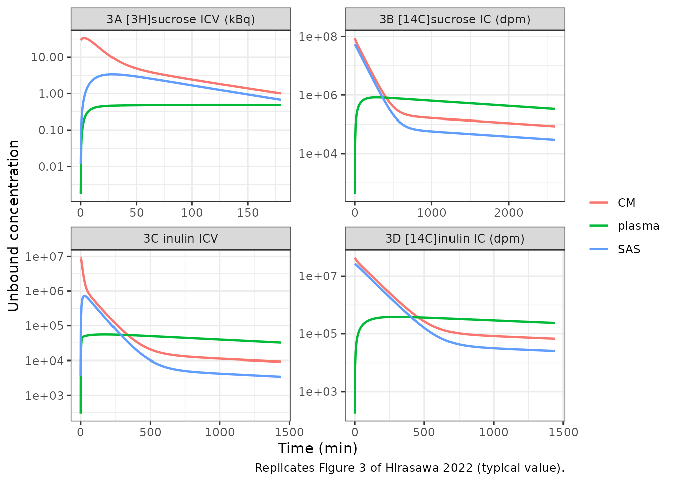
Figure 4: eight further molecules
sims |>
  filter(grepl("^4", panel)) |>
  pivot_longer(c(plasma, ECF, CM, SAS), names_to = "output", values_to = "conc") |>
  filter(conc > 1e-3) |>
  ggplot(aes(time, conc, colour = output)) +
  geom_line(linewidth = 0.8) +
  scale_y_log10() +
  facet_wrap(~panel, scales = "free", ncol = 3) +
  labs(x = "Time (min)", y = "Unbound concentration (ng/mL; nCi/mL for cefodizime)",
       colour = NULL, caption = "Replicates Figure 4 of Hirasawa 2022 (typical value).") +
  theme_bw()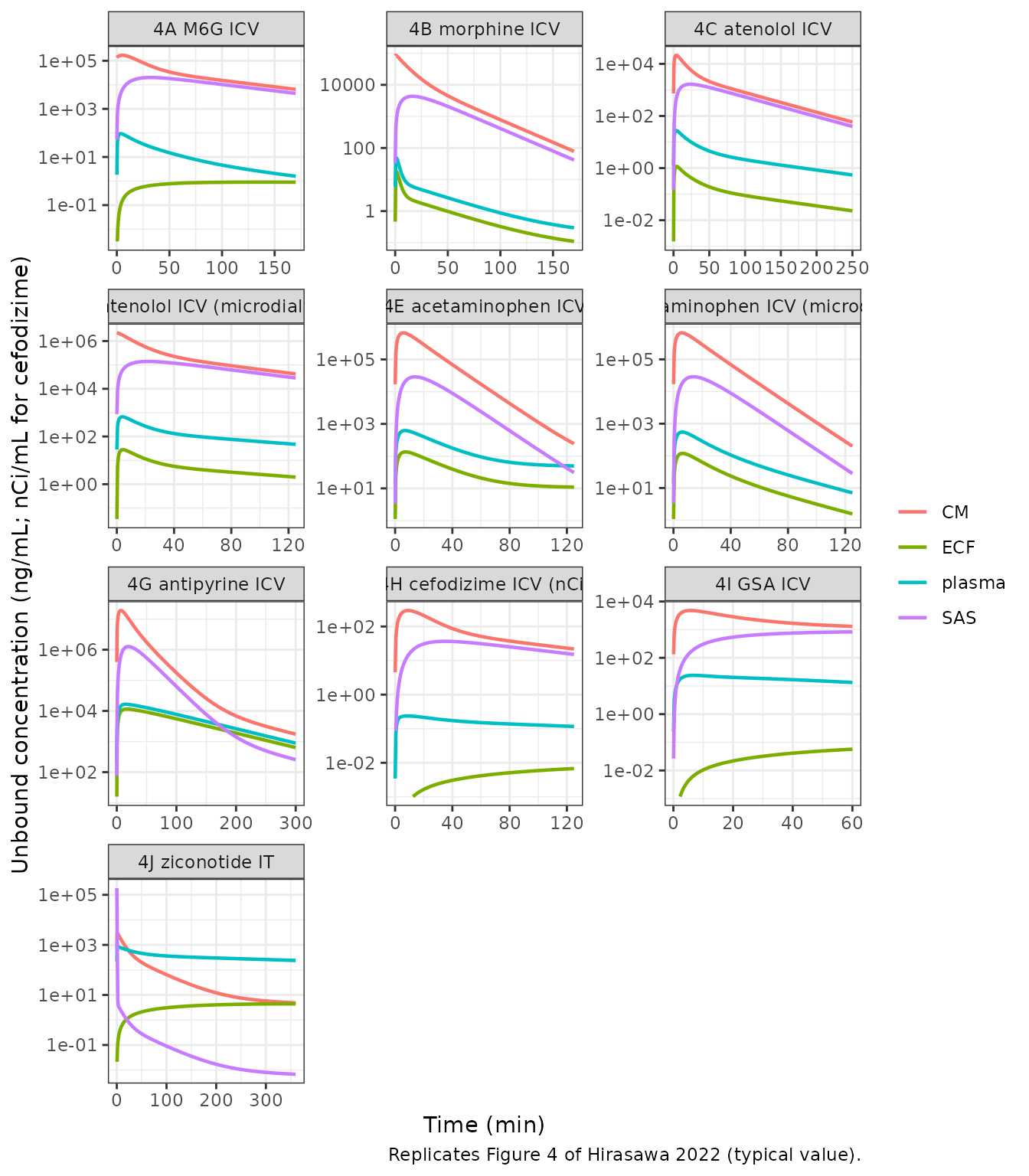
Figure 5: IV administration
sims |>
  filter(grepl("^5", panel)) |>
  pivot_longer(c(plasma, CM), names_to = "output", values_to = "conc") |>
  filter(conc > 1e-3) |>
  ggplot(aes(time, conc, colour = output)) +
  geom_line(linewidth = 0.8) +
  scale_y_log10() +
  facet_wrap(~panel, scales = "free") +
  labs(x = "Time (min)", y = "Unbound concentration", colour = NULL,
       caption = "Replicates the LeiCNS-PK3.1 columns of Figure 5 of Hirasawa 2022 (typical value).") +
  theme_bw()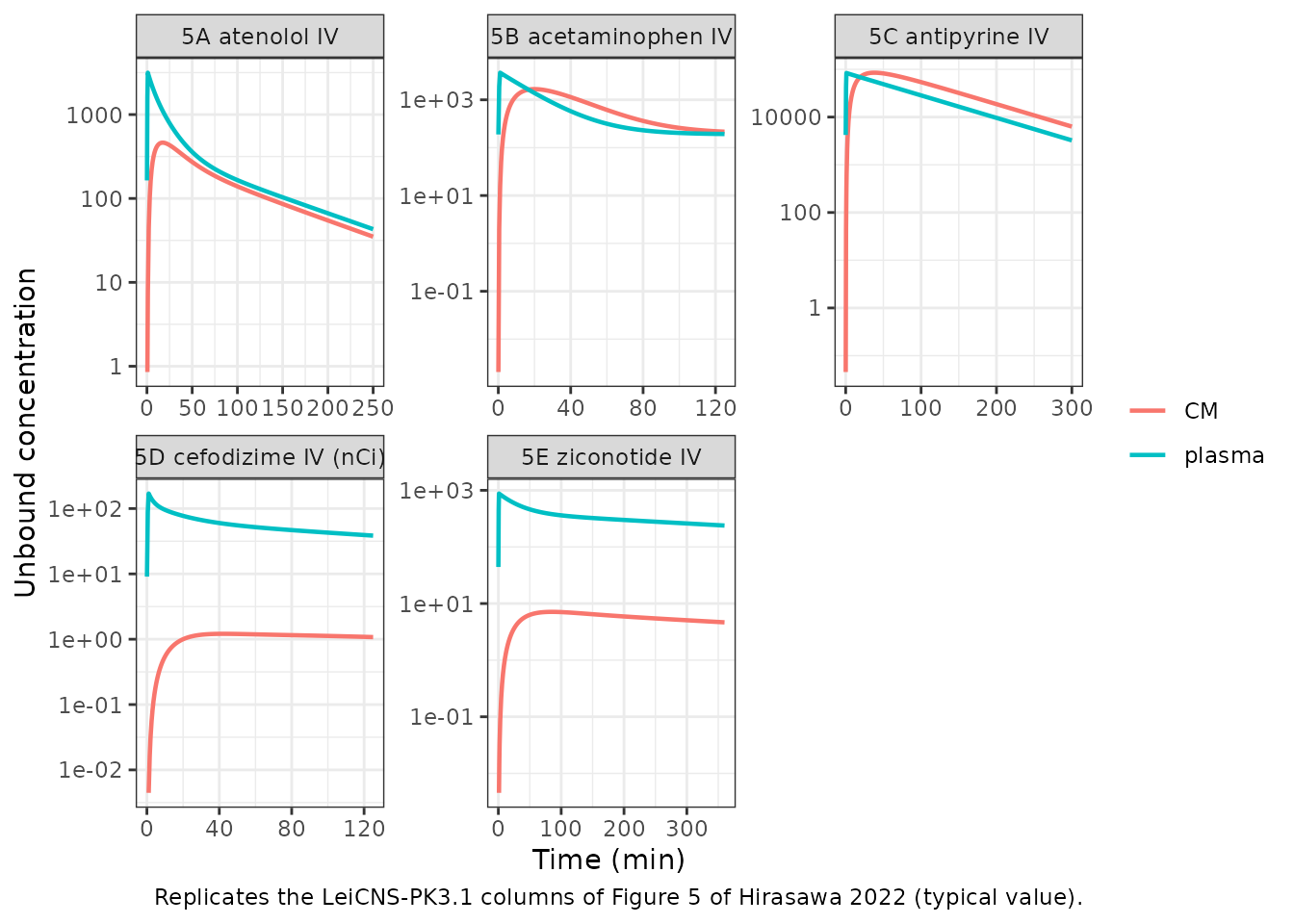
Supplementary Figures S2 and S3: structural extensions
sims |>
  filter(grepl("^S", panel)) |>
  pivot_longer(c(plasma, CM, SAS), names_to = "output", values_to = "conc") |>
  filter(conc > 1e-3) |>
  ggplot(aes(time, conc, colour = output)) +
  geom_line(linewidth = 0.8) +
  scale_y_log10() +
  facet_wrap(~panel, scales = "free") +
  labs(x = "Time (min)", y = "Unbound concentration (ng/mL)", colour = NULL,
       caption = "Replicates Supplementary Figures S2C,D and S3C,D of Hirasawa 2022.") +
  theme_bw()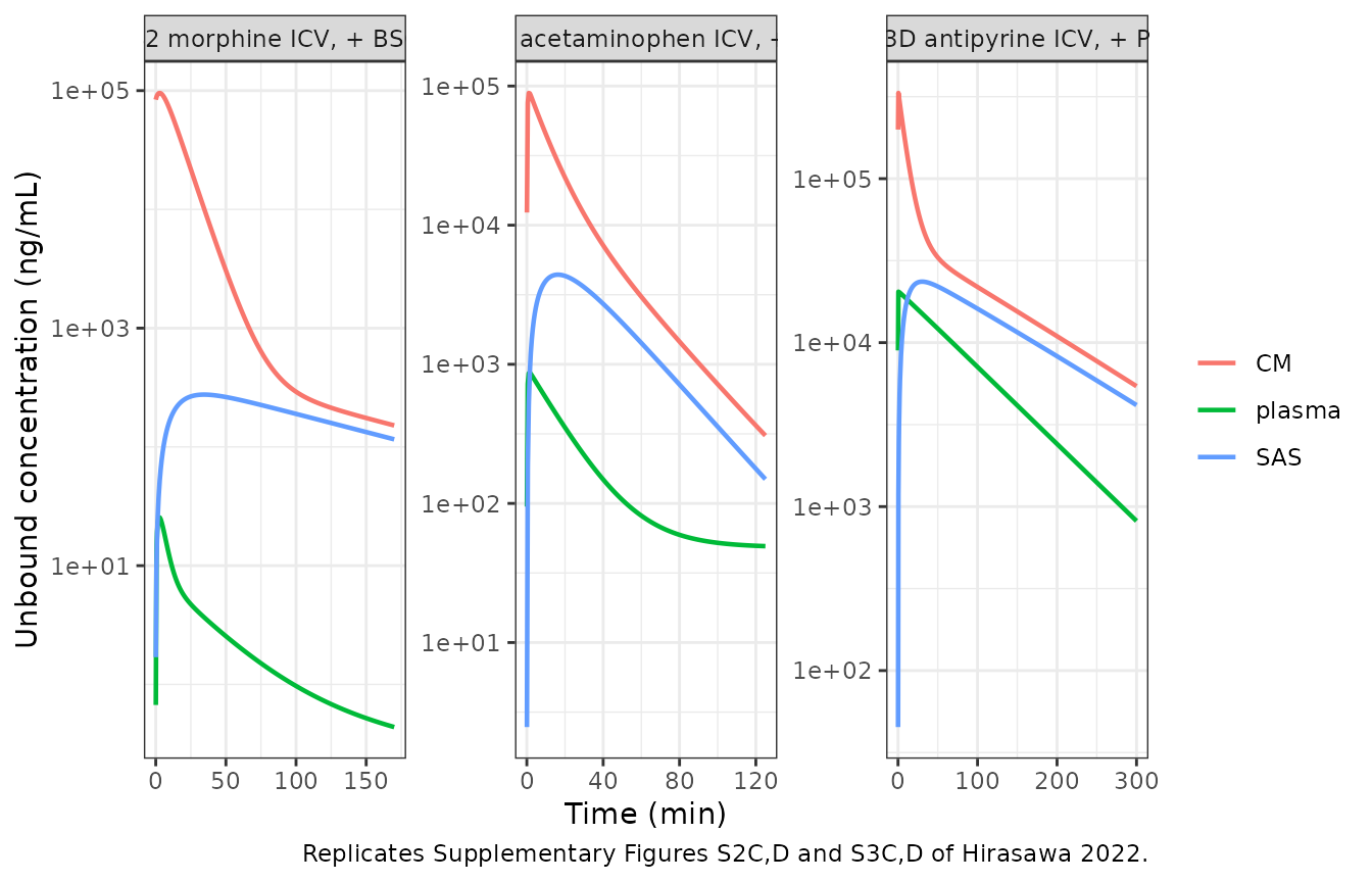
Between-subject variability: Figure 4D,F
The 95% prediction bands of Figure 4D,F come only from the IIV and residual error of the de Lange 1994 plasma models (Section 2.12). The CNS model has no variability of its own.
rxode2::rxSetSeed(20220824)
vpc <- lapply(c("4D atenolol ICV (microdialysis)", "4F acetaminophen ICV (microdialysis)"), function(p) {
  r <- scen[scen$panel == p, ]
  ev <- rxode2::et(csf_dose(r$amt, r$lv, r$tfv, r$cm, r$sas), seq(0.5, r$tend, by = 2.5))
  s <- suppressWarnings(rxode2::rxSolve(rxode2::rxode2(nlmixr2lib::readModelDb(r$model)),
                                        ev, nSub = 200, returnType = "data.frame"))
  s |>
    group_by(time) |>
    summarise(plasma_lo = quantile(sim, 0.025), plasma_med = median(Cc),
              plasma_hi = quantile(sim, 0.975),
              ecf_lo = quantile(Cbrain_ecf, 0.025), ecf_med = median(Cbrain_ecf),
              ecf_hi = quantile(Cbrain_ecf, 0.975), .groups = "drop") |>
    mutate(panel = p)
}) |>
  bind_rows()
#> ℹ parameter labels from comments will be replaced by 'label()'
#> ℹ parameter labels from comments will be replaced by 'label()'

ggplot(vpc, aes(time)) +
  geom_ribbon(aes(ymin = pmax(plasma_lo, 1e-2), ymax = plasma_hi), fill = "darkgreen", alpha = 0.2) +
  geom_line(aes(y = plasma_med, colour = "plasma")) +
  geom_ribbon(aes(ymin = ecf_lo, ymax = ecf_hi), fill = "firebrick", alpha = 0.2) +
  geom_line(aes(y = ecf_med, colour = "ECF")) +
  scale_y_log10() +
  facet_wrap(~panel, scales = "free") +
  labs(x = "Time (min)", y = "Unbound concentration (ng/mL)", colour = NULL,
       caption = "Median and 95% prediction interval of 200 simulated rats (Figure 4D,F).") +
  theme_bw()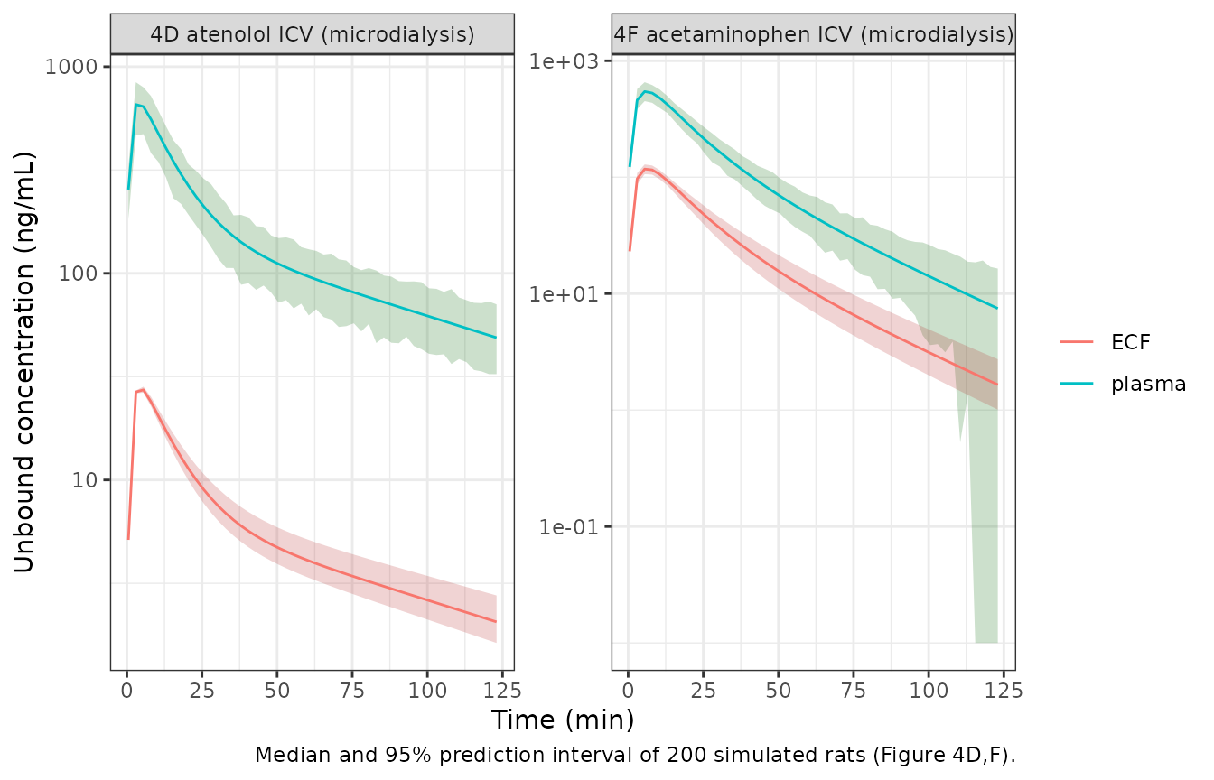
NCA of the intra-CSF profiles
The paper reports no NCA, so there is nothing to compare against. For
reference, this is a PKNCA summary of the simulated
cisterna-magna profiles after each intra-CSF dose, by panel.
cm_long <- sims |>
  filter(grepl("^[34]", panel)) |>
  transmute(panel = as.character(panel), time, conc = pmax(CM, 0)) |>
  filter(!is.na(conc))
cm_dose <- scen |>
  filter(grepl("^[34]", panel)) |>
  transmute(panel, time = 0, dose = amt)
nca_cm <- suppressWarnings(PKNCA::pk.nca(PKNCA::PKNCAdata(
  PKNCA::PKNCAconc(as.data.frame(cm_long), conc ~ time | panel),
  PKNCA::PKNCAdose(as.data.frame(cm_dose), dose ~ time | panel),
  intervals = data.frame(start = 0, end = Inf, cmax = TRUE, tmax = TRUE, auclast = TRUE)
)))
as.data.frame(nca_cm) |>
  select(panel, PPTESTCD, PPORRES) |>
  pivot_wider(names_from = PPTESTCD, values_from = PPORRES) |>
  rename("Panel" = panel, "Cmax (CM)" = cmax, "Tmax (min)" = tmax, "AUClast (CM)" = auclast) |>
  knitr::kable(digits = 3, format.args = list(scientific = 3),
caption = "Simulated cisterna-magna NCA after intra-CSF dosing (units as in each panel).")| Panel | AUClast (CM) | Cmax (CM) | Tmax (min) |
|---|---|---|---|
| 3A [3H]sucrose ICV (kBq) | 1062.239 | 33.759 | 3.000 |
| 3B [14C]sucrose IC (dpm) | 7023436874.340 | 88800000.000 | 0.000 |
| 3C inulin ICV | 260782292.833 | 9212499.029 | 0.500 |
| 3D [14C]inulin IC (dpm) | 3696602863.606 | 44400000.000 | 0.000 |
| 4A M6G ICV | 6534122.128 | 169481.032 | 4.958 |
| 4B morphine ICV | 1365528.541 | 86636.670 | 0.500 |
| 4C atenolol ICV | 504907.302 | 21384.974 | 4.167 |
| 4D atenolol ICV (microdialysis) | 40490758.560 | 2205882.353 | 0.000 |
| 4E acetaminophen ICV | 13756074.392 | 666696.418 | 5.729 |
| 4F acetaminophen ICV (microdialysis) | 13749172.341 | 666691.088 | 5.729 |
| 4G antipyrine ICV | 470024895.037 | 19117879.211 | 6.250 |
| 4H cefodizime ICV (nCi) | 10989.514 | 294.657 | 8.854 |
| 4I GSA ICV | 147696.184 | 4789.440 | 5.750 |
| 4J ziconotide IT | 53276.632 | 3037.006 | 1.000 |
Assumptions and deviations
Assumptions
- ODE equations. The paper prints no differential equations. The topology is Figure 1B, with the LeiCNS-PK3.0 parenchymal block as packaged in the Saleh 2023 mouse models. The steady state of the resulting equations reproduces the printed asymmetry-factor closed forms exactly (Gate 1). Those closed forms encode every flux, so the topology is pinned. The typical-value curves of every published panel are reproduced (Gate 4).
-
Plasma coupling. The empirical plasma model is
mass-balanced with the CNS: plasma exchanges with the brain and
choroid-plexus microvessels at
Q_CBFandQ_CPBFand receivessasQCSFfrom SAS. The LeiCNS-PK1.0 NONMEM control streams (Yamamoto 2017) are coupled the same way. Without it, drug dosed into the CSF could not reach plasma (Figures 3B,D, 4C-G, 4J). All concentrations, including those in the microvessels, are unbound. The Table S1 models describe unbound plasma data, and the closed forms contain no unbound-fraction term. - CPMV. The choroid-plexus microvessel volume and blood flow are not subtracted from the whole-brain microvessel volume and cerebral blood flow. The paper does not say, and the amounts are below 2% and 1% respectively.
- CFPPA multiplies the paracellular clearance at the BBB and at both BCSFBs (Section 2.6: “paracellular permeability (PPA) across the BBB and BCSFB”).
- BCSFB width. The Saleh 2021 table merges the BCSFB width cell with the BBB row, so both widths are 0.5 um. The BCSFB surface area (25 cm^2) is split equally between the LV and TFV barriers (Saleh 2021 footnote 13).
- IIV scale. Supplementary Table S1 gives IIV as a percentage of an exponential model. It is read as a coefficient of variation, with omega^2 = log(1 + CV^2). This affects only the prediction bands of Figure 4D,F and of the morphine model.
- Dosing. Rats weigh 250 g. Intra-CSF doses are instantaneous and split across compartments by Supplementary Table S3; the injected volume is not added to the compartment volumes. IV doses in Figure 5 are 1-min infusions (Table 1: 60 s). The [14C] doses are converted at 2.22e6 dpm/uCi.
- Units. Sucrose is in kBq (the [3H] ICV dataset). The [14C] IC dataset is in dpm and simulates identically, because the model is linear. Cefodizime is in nCi; all other molecules are in ng.
-
Asymmetry factors in the structural variants. The
paper does not say how the factors were computed for the Figure S2 and
S3 extensions. Including the added pathway in the steady state fails for
the periventricular variants: no positive choroid-plexus concentration
satisfies the reported
Kp,uu. For the BSC variant it gives curves that miss Figure S2. Applying the Supplementary Equations as printed reproduces Figures S2C,D and S3C,D (Gate 4). For the BSC variant this means usingsasQCSF,absin place ofsasQCSFand ignoring the surface compartment; for the PV variants it means ignoring the periventricular clearance. As a result, the variants’ steady-state ratios differ from Table S2 (Gate 2).
Source oddities, carried through as published
-
Supplementary Table S2 swaps the morphine and
morphine-6-glucuronide row labels. The row labelled
“Morphine-6-glucuronide” has MW 285.3, a basic charge class and logP
0.87, which is morphine (C17H19NO3, MW 285.3). The row labelled
“Morphine” has MW 461.5, zwitterion and a calculated logP of 0.13, which
is M6G (C23H27NO9, MW 461.5). Each row’s fu,
Kp,uuvalues and citations are consistent with the corrected assignment: the morphine row cites Saleh 2021 (a morphine dataset), and the M6G row cites the M6G studies of references [68-70]. Whole rows are reassigned. With this assignment the M6G and morphine panels of Figure 4A,B are reproduced (Gate 4). -
sasQCSFfor guanidinosuccinic acid is negative (-0.411 uL/min): a net influx from plasma into SAS (Table 2 and Discussion). It is kept as published. - Table 2 marks the morphine estimates (poor SAS fit) and the acetaminophen and antipyrine estimates (poor CM fit) as unsatisfactory. Supplementary Figures S2 and S3 are the authors’ attempts to fix these fits, and are packaged as separate models.
- The acetaminophen van Bree 1989 plasma model has an unusually low central clearance (0.075 mL/min) and a 4.07 L peripheral volume (Table S1). It is kept as published.