Atenolol CVS-CTR systems model (Fu 2022)
Source:vignettes/articles/Fu_2022_atenolol_qsp.Rmd
Fu_2022_atenolol_qsp.RmdModel and source
- Citation: Fu Y, Taghvafard H, Said MM, Rossman EI, Collins TA, Billiald- Desquand S, Leishman D, van der Graaf PH, van Hasselt JGC, Snelder N (2022). A novel cardiovascular systems model to quantify drugs effects on the inter-relationship between contractility and other hemodynamic variables. CPT Pharmacometrics Syst Pharmacol. 11(5):640-652. doi:10.1002/psp4.12774. Atenolol PK structure fixed from Fu 2022 Methods (Pharmacokinetic model) as cited to Venkatasubramanian 2018 and Snelder 2013. TIC = 0.256 s from Templeton 1979 (Fu 2022 reference 21).
- Article: https://doi.org/10.1002/psp4.12774
Fu et al. (2022) introduce a novel cardiovascular (CVS) systems model that integrates myocardial contractility (CTR) with the classical Snelder hemodynamic system (heart rate HR, total peripheral resistance TPR, cardiac output CO, mean arterial pressure MAP) via pressure-volume-loop (PV-loop) theory. Four indirect-response (turnover) compartments – one per hemodynamic state – are coupled by MAP feedback and by algebraic PV-loop relations that derive stroke volume, end-systolic volume, CO, and MAP from the four states plus a fixed literature-derived isovolumic contraction time. Atenolol is used as a proof-of-concept beta1-blocker (0.3-30 mg/kg PO in conscious beagle dogs); Emax inhibition of HR and CTR production shares a fixed EC50 at the literature beta1 KD (58.3 ng/mL, Baker 2005).
Population
Three in vivo telemetry studies in conscious beagle dogs contribute data:
- Study 1 (Servier, France): 4 healthy male beagles, 10-15 kg; single-dose oral atenolol at 3, 10, 30 mg/kg (or vehicle = 0.5% methylcellulose) on separate occasions; HR, dP/dtmax, cardiac output, and MAP measured over -1 to 6 h post-dose.
- Study 2 (AstraZeneca Alderley Park, UK): 4 male beagles, 14.2-14.6 kg, 17-22 months old; oral atenolol at 1, 3, 10 mg/kg (or water vehicle); HR, dP/dtmax, and MAP over -1 to 20 h post-dose (no CO measurement).
- Study 3 (GlaxoSmithKline, USA): 4 male beagles, 9-13 kg, 5-6 years old; oral atenolol at 0.3, 1, 3 mg/kg (or water vehicle); HR, dP/dtmax, and MAP. Study 3 is used only for external validation and is not encoded as a covariate level in the packaged model.
Data from Studies 1 and 2 were simultaneously fit with NONMEM 7.4.3 (FOCE-INTER) via PsN 4.8.1. Baseline HR, V0 (PV-loop x-intercept), and baseline dP/dtmax differ between studies; baseline TPR, baseline EDV, Kout, feedback strength, and the drug- effect parameters (Emax on HR and CTR) are shared. The programmatic view of the population metadata is:
readModelDb("Fu_2022_atenolol_qsp")()$population
#> $species
#> [1] "beagle dog"
#>
#> $n_subjects
#> [1] 12
#>
#> $n_studies
#> [1] 3
#>
#> $age_range
#> [1] "17-72 months (Study 1: healthy naive adult; Study 2: 17-22 months; Study 3: 5-6 years)"
#>
#> $weight_range
#> [1] "9-15 kg (Study 1: 10-15 kg; Study 2: 14.2-14.6 kg; Study 3: 9-13 kg)"
#>
#> $sex_female_pct
#> [1] 0
#>
#> $race_ethnicity
#> [1] NA
#>
#> $disease_state
#> [1] "Conscious chronically-instrumented healthy beagle dogs (male). Multi-site consortium: Servier (France; Study 1), AstraZeneca (Alderley Park, UK; Study 2), GlaxoSmithKline (Marshall Farms, NY, USA; Study 3, external validation). Hemodynamic markers monitored by telemetry: aortic and left-atrial pressures, LV pressure via solid-state micromanometer, aortic blood flow via transit-time flowmeter (Study 1) or DSI PhysioTel implants (Studies 2 and 3)."
#>
#> $dose_range
#> [1] "Oral gavage; increasing atenolol doses with washout in between: 0/3/10/30 mg/kg (Study 1, vehicle = 0.5 percent methylcellulose); 0/1/3/10 mg/kg (Study 2, vehicle = water); 0/0.3/1/3 mg/kg (Study 3, vehicle = water). Studies 1 and 2 used for model development; Study 3 for external validation."
#>
#> $regions
#> [1] "France (Servier), United Kingdom (AstraZeneca Alderley Park), USA (GlaxoSmithKline)."
#>
#> $notes
#> [1] "Data from three in vivo telemetry studies (Fu 2022 Table 1 and supplement Section A). Only HR, LV dP/dtmax, CO (Studies 1 and 3 only), and MAP time courses were used. Data from Studies 1 and 2 were simultaneously fit with NONMEM 7.4.3 (FOCE-INTER) via PsN 4.8.1. Model was initialised at 0 h and dosing began at 168 h in the fitting run so that the circadian rhythms were in oscillating steady state; for typical-user simulations the packaged model starts the CVS states at their baseline values with the circadian phase set so that t = 0 corresponds to the model's dosing time. Study 1 data used for external comparison of the developed model to CO-informative telemetry; the paper additionally fit a Model without CO data (with BSL_TPR fixed to 0.0743 mmHg*min/mL, IIV on BSL_TPR and CS_TPR removed, and Emax_TPR retained at zero) -- the packaged model corresponds to the primary Fu 2022 Table 2 final model with CO data."
Source trace
Every ini() value is annotated inline with a source
location in
inst/modeldb/specificDrugs/Fu_2022_atenolol_qsp.R. The
summary table below collects the per-parameter provenance for review;
every one of the 36 parameter values matches a number printed in the
paper.
| Group | Parameter | Value | Source location |
|---|---|---|---|
| Atenolol PK (fixed) | ka | 1.13 /h | Fu 2022 Methods p.641 ‘Pharmacokinetic model’ |
| Atenolol PK (fixed) | CL | 3.35 L/(kg*h) | Fu 2022 Methods p.641 |
| Atenolol PK (fixed) | Vc = V2 | 4.05 L/kg | Fu 2022 Methods p.641 |
| Atenolol PK (fixed) | Q = Q2 | 8.85 L/(kg*h) | Fu 2022 Methods p.641 |
| Atenolol PK (fixed) | Vp = V3 | 3.74 L/kg | Fu 2022 Methods p.641 |
| Atenolol PK (fixed) | Q2 = Q3 | 5.73 L/(kg*h) | Fu 2022 Methods p.641 |
| Atenolol PK (fixed) | Vp2 = V4 | 11.9 L/kg | Fu 2022 Methods p.641 |
| Atenolol PK (fixed) | F1 | 0.783 | Fu 2022 Methods p.641 |
| CVS baselines (S1) | BSL_HR | 79.4 beats/min | Fu 2022 Table 2 (S1 col) |
| CVS baselines (S1) | V0 | 9.92 mL | Fu 2022 Table 2 (S1 col) |
| CVS baselines (S1) | BSL_CTRM | 3777 mmHg/s | Fu 2022 Table 2 (S1 col) |
| CVS baselines (S2) | BSL_HR | 77.0 beats/min | Fu 2022 Table 2 (S2 col) |
| CVS baselines (S2) | V0 | 9.15 mL | Fu 2022 Table 2 (S2 col) |
| CVS baselines (S2) | BSL_CTRM | 2422 mmHg/s | Fu 2022 Table 2 (S2 col) |
| Shared CVS system | BSL_TPR | 0.0743 mmHg*min/mL | Fu 2022 Table 2 |
| Shared CVS system | BSL_EDV | 31.13 mL (fixed) | Fu 2022 Table 2 (fixed; ref 29) |
| Shared CVS system | Kout | 0.830 /h | Fu 2022 Table 2 (footnote a: shared HR/EDV/TPR/CTR) |
| Shared CVS system | FB | 0.00558 /mmHg | Fu 2022 Table 2 |
| Physiologic (fixed) | TIC | 0.256 s | Templeton 1979 (Fu 2022 ref 21) |
| Circadian S1 | Amp | 0.0931 | Fu 2022 Table 2 (S1 col) |
| Circadian S1 | Hor_HR | 7.86 h | Fu 2022 Table 2 (S1 col) |
| Circadian S1 | Hor_CTR | 9.82 h | Fu 2022 Table 2 (S1 col) |
| Circadian S2 | Amp | 0.168 | Fu 2022 Table 2 (S2 col) |
| Circadian S2 | Hor_HR | 19.4 h | Fu 2022 Table 2 (S2 col) |
| Circadian S2 | Hor_CTR | 21.8 h | Fu 2022 Table 2 (S2 col) |
| Circadian shared | Hor_TPR | 6.33 h (8h period) | Fu 2022 Table 2 |
| Drug effects | Emax_HR | 0.415 | Fu 2022 Table 2 |
| Drug effects | EC50_HR | 58.3 ng/mL (fixed) | Fu 2022 Table 2; Baker 2005 (ref 23) |
| Drug effects | Emax_CTR | 0.422 | Fu 2022 Table 2 |
| Drug effects | EC50_CTR | 58.3 ng/mL (fixed) | Fu 2022 Table 2 (= EC50_HR, THETA(11)=1 FIX) |
| IIV | omega(BSL_HR) | CV% 6.08 | Fu 2022 Table 2 |
| IIV block | omega(BSL_TPR, BSL_CTRM) | CV% 6.48 / 16.58, off-diag 8.88 | Fu 2022 Table 2 |
| Residual (lnorm) | expSd_HR | 0.115 (CV% approx 11.53) | Fu 2022 Table 2 |
| Residual (lnorm) | expSd_CTRM | 0.104 (CV% approx 10.43) | Fu 2022 Table 2 |
| Equation (Eq 1) | MAP = TPR * CO; CO = HR * SV | n/a | Fu 2022 Methods |
| Equation (Eq 2) | SV = EDV - ESV | n/a | Fu 2022 Methods |
| Equation (Eq 4) | EA = HR * TPR | n/a | Fu 2022 Methods |
| Equation (Eq 6) | ESV = (EDVEA + V0CTR)/(EA+CTR) | n/a | Fu 2022 Methods |
| Equation (Eq 7) | CTRM = CTR * EDV / TIC | n/a | Fu 2022 Methods |
| Equation (Eq 8) | 4 turnover ODEs w/ (1+CS)(1-FDB)(1-EFF) | n/a | Fu 2022 Methods and CTL $DES |
Simulation setup
The paper uses a 1-week warm-up (system initialized at t = 0 h;
dosing at t = 168 h) so that the circadian rhythm reaches oscillating
steady state before the drug is administered. The packaged model mirrors
this convention: dose at t = 168 and observe over the
following 24 h.
Cohort size is capped at 25 per dose group (100 subjects total). The paper’s real n is 4 per dose; a virtual cohort of 25 gives smooth prediction intervals without inflating render time.
build_cohort <- function(dose_mg_per_kg, n, id_offset, study_az = 0L) {
  # A per-subject event table: single oral dose at t = 168 h (matches the
  # Fu 2022 simulation convention -- 1-week warm-up so the circadian rhythm
  # reaches oscillating steady state before dosing).
  ids  <- id_offset + seq_len(n)
  tobs <- seq(from = 168, to = 168 + 24, by = 0.25)
  treatment_lbl <- if (dose_mg_per_kg > 0)
    paste0(format(dose_mg_per_kg), " mg/kg") else "vehicle"

  # Build via rxode2::et(). The model declares two endpoints (HR and CTRM);
  # observation rows carry `cmt = "HR"` to identify the primary endpoint (a
  # requirement of the multi-endpoint rxode2 event grammar). rxSolve returns
  # HR, CTRM, CO, MAP, Cc, and all ODE states as columns regardless of the
  # observation `cmt` value.
  dplyr::bind_rows(lapply(ids, function(sid) {
    # Units are recorded STATICALLY in the comments below (and canonically in
    # the model's own `units` field: time = hours, dosing = mg/kg) rather than
    # declared via et(amountUnits=, timeUnits=). Those arguments attach unit
    # attributes through the `units` package, which is NOT a dependency of
    # nlmixr2lib and is absent on the CI runners -- pkgdown failed with
    # "there is no package called 'units'". Nothing was gained by declaring
    # them here: the attributes were stripped back to plain numerics two lines
    # later so dplyr::bind_rows could align the columns. No unit CONVERSION is
    # performed anywhere in this vignette; every dose is already mg/kg and
    # every time is already hours, matching the model.
    ev <- rxode2::et()
    if (dose_mg_per_kg > 0) {
      # amt in mg/kg; time in hours (dose at 168 h = end of the 1-week warm-up)
      ev <- ev |>
        rxode2::et(amt = dose_mg_per_kg, cmt = "depot", time = 168)
    }
    ev <- ev |> rxode2::et(time = tobs, cmt = "HR")   # tobs in hours
    df <- as.data.frame(ev)
    df$id              <- sid
    df$STUDY_FU2022_AZ <- study_az
    df$treatment       <- treatment_lbl
    df
  }))
}

events <- dplyr::bind_rows(
  build_cohort(0,  n = 25L, id_offset =   0L, study_az = 0L),
  build_cohort(3,  n = 25L, id_offset =  25L, study_az = 0L),
  build_cohort(10, n = 25L, id_offset =  50L, study_az = 0L),
  build_cohort(30, n = 25L, id_offset =  75L, study_az = 0L)
) |>
  dplyr::mutate(
    treatment = factor(treatment,
                       levels = c("vehicle", "3 mg/kg", "10 mg/kg", "30 mg/kg"))
  )

stopifnot(!anyDuplicated(unique(events[, c("id", "time", "evid")])))

# Cohort composition
events |>
  dplyr::filter(evid == 1) |>
  dplyr::count(treatment) |>
knitr::kable(caption = "Virtual cohort composition (Study 1 dose grid).")| treatment | n |
|---|---|
| 3 mg/kg | 25 |
| 10 mg/kg | 25 |
| 30 mg/kg | 25 |
Simulation
mod <- readModelDb("Fu_2022_atenolol_qsp")

sim <- rxode2::rxSolve(mod, events = events, keep = c("treatment"))
#> ℹ parameter labels from comments will be replaced by 'label()'
Steady-state check (no dose)
Under the vehicle arm the CVS states should oscillate around their published baselines (BSL_HR = 79.4 bpm, BSL_TPR = 0.0743 mmHg*min/mL, BSL_CTRM = 3777 mmHg/s, BSL_EDV = 31.13 mL, BSL_MAP approx 105 mmHg). Deviations are due to the circadian rhythm and inter-individual variability only.
vehicle_summary <- sim |>
  dplyr::filter(treatment == "vehicle") |>
  dplyr::group_by(time) |>
  dplyr::summarise(
    HR_med   = median(HR),
    MAP_med  = median(MAP),
    CTRM_med = median(CTRM),
    CO_med   = median(CO),
    .groups  = "drop"
  )

tibble::tibble(
  Metric     = c("Median HR (bpm)", "Median MAP (mmHg)",
                 "Median dP/dtmax (mmHg/s)", "Median CO (mL/min)"),
  `Baseline (paper)` = c("79.4", "approx 105", "3777", "approx 1415"),
  `Sim median (t = 168 h)` = c(
    sprintf("%.1f", vehicle_summary$HR_med[which.min(abs(vehicle_summary$time - 168))]),
    sprintf("%.1f", vehicle_summary$MAP_med[which.min(abs(vehicle_summary$time - 168))]),
    sprintf("%.0f", vehicle_summary$CTRM_med[which.min(abs(vehicle_summary$time - 168))]),
    sprintf("%.0f", vehicle_summary$CO_med[which.min(abs(vehicle_summary$time - 168))])
  )
) |>
  knitr::kable(align = "lrr",
               caption = paste("Steady-state (vehicle, t = 168 h) medians vs.",
"published Study 1 baselines."))| Metric | Baseline (paper) | Sim median (t = 168 h) |
|---|---|---|
| Median HR (bpm) | 79.4 | 80.4 |
| Median MAP (mmHg) | approx 105 | 105.2 |
| Median dP/dtmax (mmHg/s) | 3777 | 3590 |
| Median CO (mL/min) | approx 1415 | 1399 |
Atenolol PK profile
Before evaluating the hemodynamic response, verify that the fixed three-compartment PK reproduces reasonable atenolol plasma-concentration profiles. Figure S7 of Fu 2022 shows atenolol PK following single oral doses of 0.3, 1, 3, 10, and 30 mg/kg; peak Cc scales linearly with dose (single-compartment linear PK in beagle).
sim |>
  dplyr::filter(treatment != "vehicle", time >= 168) |>
  dplyr::mutate(time_post_dose = time - 168) |>
  dplyr::group_by(treatment, time_post_dose) |>
  dplyr::summarise(
    Q05 = quantile(Cc, 0.05, na.rm = TRUE),
    Q50 = quantile(Cc, 0.50, na.rm = TRUE),
    Q95 = quantile(Cc, 0.95, na.rm = TRUE),
    .groups = "drop"
  ) |>
  ggplot(aes(time_post_dose, Q50, colour = treatment, fill = treatment)) +
  geom_ribbon(aes(ymin = Q05, ymax = Q95), alpha = 0.15, colour = NA) +
  geom_line(linewidth = 0.7) +
  scale_y_log10() +
  labs(x = "Time post-dose (h)", y = "Atenolol Cc (ng/mL)",
       colour = "Dose", fill = "Dose",
       title = "Simulated atenolol plasma concentration",
       caption = "Fixed 3-compartment PK from Fu 2022 Methods 'Pharmacokinetic model' paragraph.") +
  geom_hline(yintercept = 58.3, linetype = "dashed", colour = "grey40") +
  annotate("text", x = 20, y = 65, hjust = 1, size = 3,
           label = "beta1 KD = 58.3 ng/mL")
#> Warning in scale_y_log10(): log-10 transformation introduced infinite values.
#> log-10 transformation introduced infinite values.
#> log-10 transformation introduced infinite values.
#> log-10 transformation introduced infinite values.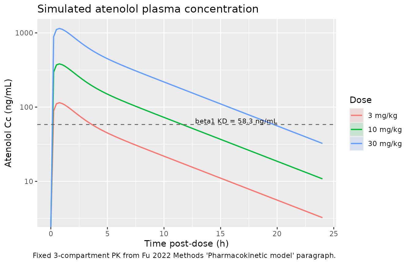
NCA on the simulated atenolol PK
The paper does not publish an NCA table for atenolol, but PKNCA provides an easy sanity check that the fixed PK behaves reasonably. Cmax should be well above the beta1 KD (58.3 ng/mL) at the 3 mg/kg and higher dose levels and below/near the KD at 0.3-1 mg/kg (consistent with Figure S7).
sim_nca <- sim |>
  dplyr::filter(treatment != "vehicle") |>
  dplyr::mutate(time_pd = time - 168) |>
  dplyr::filter(!is.na(Cc), time_pd >= 0) |>
  dplyr::select(id, time_pd, Cc, treatment) |>
  dplyr::rename(time = time_pd)

# Guarantee a time = 0 row per (id, treatment) with Cc = 0 (pre-dose).
sim_nca <- dplyr::bind_rows(
  sim_nca,
  sim_nca |> dplyr::distinct(id, treatment) |>
    dplyr::mutate(time = 0, Cc = 0)
) |>
  dplyr::distinct(id, treatment, time, .keep_all = TRUE) |>
  dplyr::arrange(id, treatment, time)

conc_obj <- PKNCA::PKNCAconc(sim_nca, Cc ~ time | treatment + id)

dose_df <- events |>
  dplyr::filter(evid == 1, treatment != "vehicle") |>
  dplyr::mutate(time = 0) |>
  dplyr::select(id, time, amt, treatment)

dose_obj <- PKNCA::PKNCAdose(dose_df, amt ~ time | treatment + id)

intervals <- data.frame(
  start = 0, end = 24,
  cmax  = TRUE, tmax = TRUE, auclast = TRUE, half.life = TRUE
)

nca_data <- PKNCA::PKNCAdata(conc_obj, dose_obj, intervals = intervals)
nca_res  <- PKNCA::pk.nca(nca_data)

as.data.frame(nca_res) |>
  dplyr::group_by(treatment, PPTESTCD) |>
  dplyr::summarise(median = median(PPORRES, na.rm = TRUE),
                   .groups = "drop") |>
  tidyr::pivot_wider(names_from = PPTESTCD, values_from = median) |>
  dplyr::rename("Dose"           = treatment,
                "Cmax (ng/mL)"   = cmax,
                "Tmax (h)"       = tmax,
                "AUC0-24 (ng*h/mL)" = auclast,
                "t1/2 (h)"       = half.life) |>
  knitr::kable(digits = c(0, 1, 2, 0, 2),
caption = "Simulated atenolol NCA (median across 25 virtual dogs per arm).")| Dose | adj.r.squared | AUC0-24 (ng*h/mL) | clast.pred | Cmax (ng/mL) | t1/2 (h) | lambda.z | lambda.z.n.points | lambda.z.time.first | lambda.z.time.last | r.squared | span.ratio | tlast | Tmax (h) |
|---|---|---|---|---|---|---|---|---|---|---|---|---|---|
| 3 mg/kg | 1 | 673.95 | 3 | 114.69 | 5 | 0.1 | 78 | 5 | 24 | 1 | 3.8 | 24 | 1 |
| 10 mg/kg | 1 | 2246.49 | 11 | 382.29 | 5 | 0.1 | 78 | 5 | 24 | 1 | 3.8 | 24 | 1 |
| 30 mg/kg | 1 | 6739.48 | 32 | 1146.87 | 5 | 0.1 | 78 | 5 | 24 | 1 | 3.8 | 24 | 1 |
Figure 3 replication: Hemodynamic VPCs by dose
Figure 3 of Fu 2022 shows visual predictive checks (VPCs) of HR, dP/dtmax, CO, and MAP under placebo and 3, 10, 30 mg/kg atenolol (Study 1). The plot below reproduces the shape of the response with the packaged model.
long <- sim |>
  dplyr::filter(time >= 168) |>
  dplyr::mutate(time_pd = time - 168) |>
  dplyr::select(id, time_pd, treatment, HR, CTRM, CO, MAP) |>
  tidyr::pivot_longer(cols = c(HR, CTRM, CO, MAP),
                      names_to = "endpoint", values_to = "value") |>
  dplyr::mutate(endpoint = factor(endpoint,
                                  levels = c("HR", "CTRM", "CO", "MAP"),
                                  labels = c("HR (bpm)", "dP/dtmax (mmHg/s)",
                                             "CO (mL/min)", "MAP (mmHg)")))

vpc <- long |>
  dplyr::group_by(endpoint, treatment, time_pd) |>
  dplyr::summarise(
    Q05 = quantile(value, 0.05, na.rm = TRUE),
    Q50 = quantile(value, 0.50, na.rm = TRUE),
    Q95 = quantile(value, 0.95, na.rm = TRUE),
    .groups = "drop"
  )

ggplot(vpc, aes(time_pd, Q50, colour = treatment, fill = treatment)) +
  geom_ribbon(aes(ymin = Q05, ymax = Q95), alpha = 0.15, colour = NA) +
  geom_line(linewidth = 0.6) +
  facet_wrap(~ endpoint, scales = "free_y") +
  labs(x = "Time post-dose (h)", y = NULL,
       colour = "Dose", fill = "Dose",
       title = "Replicates Figure 3 of Fu 2022 (Study 1 CVS-CTR VPC)",
       caption = paste("Virtual population n = 25 per dose; ribbons = 5th-95th",
                       "prediction percentile; lines = median. Dose applied at",
                       "the model's t = 168 h (=0 h post-dose)."))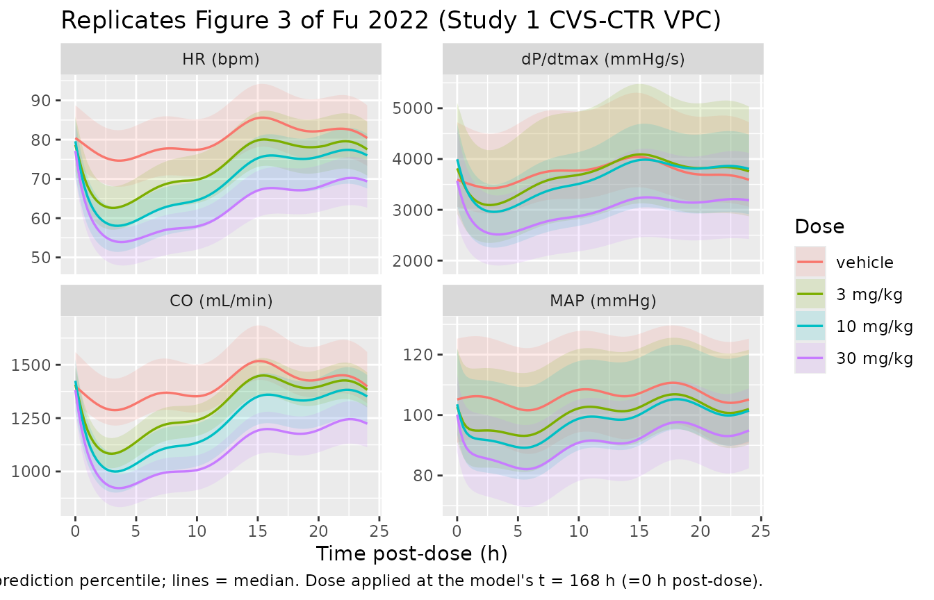
The expected direction of effect: increasing atenolol dose produces a dose-dependent DROP in HR and dP/dtmax (both beta1-mediated), a MODEST drop in CO (HR falls faster than SV rises), and a smaller drop in MAP (partially compensated by MAP-mediated feedback that up-regulates HR / TPR / CTR production).
Study 2 comparison
Study 2 (AstraZeneca, STUDY_FU2022_AZ = 1) has slightly
lower baseline HR (77.0 vs 79.4 bpm), lower baseline dP/dtmax (2422 vs
3777 mmHg/s), and larger circadian amplitude (0.168 vs 0.0931). The
packaged model reproduces both studies with the same shared drug-effect
parameters.
events_s2 <- dplyr::bind_rows(
  build_cohort(0,  n = 25L, id_offset =   0L, study_az = 1L),
  build_cohort(1,  n = 25L, id_offset =  25L, study_az = 1L),
  build_cohort(3,  n = 25L, id_offset =  50L, study_az = 1L),
  build_cohort(10, n = 25L, id_offset =  75L, study_az = 1L)
) |>
  dplyr::mutate(
    treatment = factor(treatment,
                       levels = c("vehicle", "1 mg/kg", "3 mg/kg", "10 mg/kg"))
  )
stopifnot(!anyDuplicated(unique(events_s2[, c("id", "time", "evid")])))

sim_s2 <- rxode2::rxSolve(mod, events = events_s2, keep = c("treatment"))

sim_s2 |>
  dplyr::filter(time >= 168) |>
  dplyr::mutate(time_pd = time - 168) |>
  dplyr::select(time_pd, treatment, HR, CTRM, MAP) |>
  tidyr::pivot_longer(cols = c(HR, CTRM, MAP),
                      names_to = "endpoint", values_to = "value") |>
  dplyr::mutate(endpoint = factor(endpoint,
                                  levels = c("HR", "CTRM", "MAP"),
                                  labels = c("HR (bpm)", "dP/dtmax (mmHg/s)",
                                             "MAP (mmHg)"))) |>
  dplyr::group_by(endpoint, treatment, time_pd) |>
  dplyr::summarise(Q50 = median(value, na.rm = TRUE), .groups = "drop") |>
  ggplot(aes(time_pd, Q50, colour = treatment)) +
  geom_line(linewidth = 0.6) +
  facet_wrap(~ endpoint, scales = "free_y") +
  labs(x = "Time post-dose (h)", y = "Median",
       colour = "Dose",
       title = "Study 2 (AstraZeneca) typical-value trajectories",
       caption = "STUDY_FU2022_AZ = 1; median across 25 virtual dogs per dose.")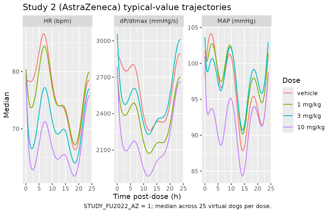
Assumptions and deviations
-
Circadian phase. The packaged model initializes the
CVS states at exact baseline (
hr(0) <- bsl_hr, etc.) and applies the circadian rhythm from t = 0. The vignette follows the paper’s t = 168 h dosing convention so the circadian rhythm reaches oscillating steady state before the drug is applied. Users may either preserve this convention or dose at t = 0 with an expected small transient over the first Kout half-life (approx 0.83 h) as the states adjust to the initial circadian phase. - Cohort size. Simulations use n = 25 virtual dogs per dose group vs. n = 4 real dogs per dose in the paper. This gives smooth prediction intervals without inflating render time.
- CO / MAP residual error. The source CTL propagates the HR and dP/dtmax residuals through the algebraic PV-loop identities to compute residuals on CO and MAP; TPR residual is FIXED at 0. The packaged model applies log-normal residual error only on HR and CTRM directly; simulated CO and MAP inherit the variability of their upstream states but do not carry an independent residual layer. This is appropriate for VPC-style validation (the primary use case); refitting CO or MAP jointly would require restoring the propagated-residual structure.
-
Study 3 external-validation cohort. Study 3
(GlaxoSmithKline, 0.3/1/3 mg/kg) is not encoded as a separate covariate
level; for Study-3-style external simulations, use
STUDY_FU2022_AZ = 0with the Study 1 baselines and interpret the results as Servier-baseline-anchored predictions. - BSL_EDV literature source. The Fu 2022 Discussion attributes the 31.13 mL BSL_EDV value to reference 29 of the paper (not available when this model was built; the value is a reported literature typical for beagle end-diastolic volume). Fixed as stated in Table 2.
-
Amp_TPR = per-study Amp (both studies). The Fu 2022
Table 2 footnote reads “AmpHR = AmpCTR = AmpTPR = Amp, Amp_1 and Amp_2
are the amplitudes of circadian rhythm for studies 1 and 2 respectively,
and for TPR the Amp and Hor were assumed to be the same as in study 1.”
The CTL implements
AMP3 = AMP1 * THETA(30)withTHETA(30) = 1 FIX– meaning AMP_TPR takes the current study’s AMP1. The packaged model follows the CTL (AMP_TPR = the per-study Amp); this deviates from the strict reading of the footnote, which would keep AMP_TPR at the Study-1 value in both studies. Users who need the footnote-strict behaviour should hard-code AMP_TPR toexp(lamp_s1)in a downstream edit. - TPR residual = 0 FIX. The paper reports “The residual error of TPR was very small and, therefore, it was fixed to 0.” The packaged model matches (no expSd_TPR entry).
-
Emax_TPRrejected. A positive TPR effect (beta2-mediated) was added in an early model iteration but rejected: “the final estimate of Emax for TPR approached zero, and the OFV did not decrease significantly”. The packaged model does not include a drug effect on TPR. Users who want to simulate a hypothetical beta2 effect can inject a(1 + Emax_TPR * Cc / (EC50_TPR + Cc))factor intod/dt(tpr)by editing the model source.