Long-acting injectable nevirapine (Cortez 2015) • nlmixr2lib

Model and source

Cortez 2015 develops the first injectable, sustained-release nevirapine (NVP) formulations intended to replace the 4-to-6 week daily oral NVP prophylaxis regimen that the WHO recommends for breastfeeding infants of HIV-1-infected mothers. Two candidate formulations (NVP LA-1 and NVP LA-2) were dosed subcutaneously to Sprague-Dawley rats in two separate studies, a population PK model was fitted to each rat data set by naive pooling in Phoenix NLME, and the rat-derived presystemic release kinetics were then combined with published breastfeeding-infant systemic PK to project human infant exposure.

The paper therefore contains four distinct models, and the extraction ships four model files:

model_names <- c(
  "Cortez_2015_nevirapine_rat_la1",
  "Cortez_2015_nevirapine_rat_la2",
  "Cortez_2015_nevirapine_human_la1",
  "Cortez_2015_nevirapine_human_la2"
)
uis <- lapply(model_names, function(n) rxode2::rxode(readModelDb(n)))
names(uis) <- model_names

tibble::tibble(
  Model     = model_names,
  Structure = c("Rat, 2-cmt, 1st-order absorption, linear elimination",
                "Rat, 1-cmt, 1st-order absorption, elimination from Vm/Km",
                "Infant, 2-cmt, human Vc/CL + rat-scaled ka/Vp/CLp",
                "Infant, 1-cmt, human V/CL + rat-scaled ka"),
  Figure    = c("Figure 3A", "Figure 3B", "Figure 4A, 4B", "Figure 4C, 4D")
) |>
  knitr::kable(caption = "The four models Cortez 2015 contributes.")

The four models Cortez 2015 contributes.
Model	Structure	Figure
Cortez_2015_nevirapine_rat_la1	Rat, 2-cmt, 1st-order absorption, linear elimination	Figure 3A
Cortez_2015_nevirapine_rat_la2	Rat, 1-cmt, 1st-order absorption, elimination from Vm/Km	Figure 3B
Cortez_2015_nevirapine_human_la1	Infant, 2-cmt, human Vc/CL + rat-scaled ka/Vp/CLp	Figure 4A, 4B
Cortez_2015_nevirapine_human_la2	Infant, 1-cmt, human V/CL + rat-scaled ka	Figure 4C, 4D

Citation: Cortez JM Jr, Quintero R, Moss JA, Beliveau M, Smith TJ, Baum MM. Pharmacokinetics of injectable, long-acting nevirapine for HIV prophylaxis in breastfeeding infants. Antimicrob Agents Chemother. 2015;59(1):59-66. doi:10.1128/AAC.03906-14.
Article: https://doi.org/10.1128/AAC.03906-14

All four model files declare time = "day", dosing = "mg" and concentration = "ug/mL". A dose in mg divided by a volume in L is mg/L, and mg/L is numerically identical to ug/mL, so Cc is directly in ug/mL. The paper plots concentrations in ng/mL, so the figures below multiply Cc by 1000.

Two published results are not reproducible, and are gated as known deviations

This vignette reproduces the LA-1 arm (Figures 3A, 4A and 4B) closely. The LA-2 arm does not reproduce, for reasons that are properties of the publication rather than of the transcription, and both are quantified below rather than tuned away:

The LA-2 rat elimination is under-determined. The Discussion says the study 2 formulation needed “saturable elimination”, but Table 2 reports one number for it – CL/F = 48.2 L/day, footnoted as the intrinsic clearance Vm/Km. Vm and Km are never reported separately, and Vm*C/(Km + C) needs both. The model file encodes the exact C << Km limit of that term (first-order elimination at CL/F = 48.2 L/day), which uses the published number and invents nothing, but does not reproduce the saturation.
Figure 4C and 4D are inconsistent with the paper’s own stated systemic parameters. The Methods give V/F = 20.0 L, CL/F = 0.21 L/h and t1/2 = 66 h, which are mutually consistent. Figures 4C and 4D start at 60 mg / 20 L = 3.0 ug/mL, confirming V/F = 20 L was used, but then decay with an apparent half-life near 66 days rather than 66 hours.

Population

Rat study 1 (JNN00006, March 2006) dosed n = 4 Sprague-Dawley rats of mean weight 0.33 kg with a single 60 mg subcutaneous injection of the NVP LA-1 microparticle suspension in 1 mL saline through a 14-gauge needle. Because of injection inefficiencies the authors modelled the delivered dose as 75% of nominal, i.e. 45 mg (135 mg/kg). Sampling was on days 1 (1 and 6 h post-dose), 2, 3, 4, 6, 10, 14 and 28.

Rat study 2 (JNN00030, May 2009) dosed n = 10 Sprague-Dawley rats of mean weight 0.21 kg with a single weight-adjusted 36 mg/kg subcutaneous injection of NVP LA-2 through an 18-gauge needle; 80% delivery was assumed, i.e. 6.7 mg (29 mg/kg). Sampling was on days -7, 1 (1, 3, 7 and 12 h post-dose), 2, 3, 7, 14, 21 and 28.

Both studies assayed plasma NVP by LC-MS/MS with an LLOQ of 1 ng/mL and set BLLOQ values to missing rather than imputing them. No between-subject variability was estimated in either fit because of the small n, and the naive pooled approach was used throughout. Subcutaneous bioavailability was assumed to be 100% for both formulations.

The human projection uses infant systemic parameters “compiled from recent clinical studies in Uganda examining the population PK of single-dose NVP in breastfeeding infants of HIV-positive mothers”: V/F = 20.0 L, CL/F = 0.21 L/h, t1/2 = 66 h, over a newborn weight range of 2.0 to 3.9 kg. Figure 4 simulates a single subcutaneous dose at those two weights – 200 mg of NVP LA-1 (panels A and B) and 60 mg of NVP LA-2 (panels C and D). The prophylactic window the simulation is judged against is 0.2 to 3.0 ug/mL: 0.2 ug/mL is five times the reported NVP IC90 of ~40 ng/mL, and 3.0 ug/mL is the accepted steady-state safety ceiling.

The same information is available programmatically:

str(uis[["Cortez_2015_nevirapine_rat_la1"]]$population,   max.level = 1)
#> List of 10
#>  $ species      : chr "rat (Sprague-Dawley)"
#>  $ n_subjects   : int 4
#>  $ n_studies    : int 1
#>  $ age_range    : chr "Adult (age not reported)"
#>  $ weight_range : chr "Mean 0.33 kg (individual weights not reported)"
#>  $ weight_median: chr "0.33 kg (reported as the mean)"
#>  $ disease_state: chr "Healthy"
#>  $ dose_range   : chr "Single 60 mg subcutaneous injection of NVP LA-1 suspended in 1 mL saline through a 14-gauge needle. Cortez 2015"| __truncated__
#>  $ regions      : chr "United States (Charles River Laboratories, Shrewsbury, MA)"
#>  $ notes        : chr "Study 1 (JNN00006, March 2006). Serial jugular-vein sampling on days 1 (1 and 6 h post-dose), 2, 3, 4, 6, 10, 1"| __truncated__
str(uis[["Cortez_2015_nevirapine_human_la1"]]$population, max.level = 1)
#> List of 9
#>  $ species      : chr "human"
#>  $ n_subjects   : int NA
#>  $ n_studies    : int 2
#>  $ age_range    : chr "Neonates from birth (WHO prophylaxis window is birth to 4-6 weeks of age)"
#>  $ weight_range : chr "2.0-3.9 kg"
#>  $ disease_state: chr "HIV-uninfected breastfeeding infants born to HIV-1-infected mothers, receiving nevirapine as prophylaxis agains"| __truncated__
#>  $ dose_range   : chr "Single 200 mg subcutaneous injection of NVP LA-1 (Cortez 2015 Figure 4A and 4B)"
#>  $ regions      : chr "Uganda (source of the systemic infant PK estimates)"
#>  $ notes        : chr "Cortez 2015 Methods 'Human simulations': \"Infant parameters for the human simulations were compiled from recen"| __truncated__

Source trace

Every ini() entry in all four model files carries an in-file comment naming its source location. They are collected here for review.

Model	Equation / parameter	Value	Source location
rat LA-1	`lka` (Ka)	1.89 /day	Table 2, study 1 column (RSE 26.1%)
rat LA-1	`lvc` (Vc/F)	8.66 L	Table 2, study 1 column (RSE 17.9%)
rat LA-1	`lvp` (Vp/F)	14.3 L	Table 2, study 1 column (RSE not available)
rat LA-1	`lcl` (CL/F)	3.43 L/day	Table 2, study 1 column (RSE 11.3%)
rat LA-1	`lq` (CLp/F)	0.541 L/day	Table 2, study 1 column (RSE 35.8%)
rat LA-1	`addSd`	28.6 ug/L = 0.0286 ug/mL	Table 2, study 1 `Error` row (RSE 40.4%)
rat LA-1	`propSd`	0.501	Table 2, study 1 `Error` row (RSE 32.4%)
rat LA-1	structure	2-cmt, linear absorption + elimination	Discussion: “a two-compartment model with linear absorption and linear elimination adequately described the study 1 formulation”
rat LA-2	`lka` (Ka)	15.4 /day	Table 2, study 2 column (RSE 41.8%)
rat LA-2	`lvc` (Vc/F)	74.0 L	Table 2, study 2 column (RSE 16.2%)
rat LA-2	`lcl` (CL/F)	48.2 L/day	Table 2, study 2 column (RSE 47.2%) + footnote d: “Represents intrinsic clearance (Vm/Km) …”
rat LA-2	`propSd`	0.790	Table 2, study 2 `Error` row (RSE 9.4%)
rat LA-2	structure	1-cmt, linear absorption, saturable elimination	Discussion: “a one-compartment model with linear absorption and saturable elimination adequately described the study 2 formulation”
both rat	`lfdepot` (F)	1 (fixed)	Discussion: F assumed 100% for both formulations
both rat	residual error form `y = yhat*(1+eps1) + eps2`	n/a	Methods equation 2
all	`e_wt_ka` / `e_wt_vc` / `e_wt_vp` / `e_wt_cl` / `e_wt_q`	-0.25 / 1 / 1 / 0.75 / 0.75 (fixed)	Methods, “Structural PK model buildup”: “The nominal covariate effect was -0.25 on absorption rate, 1 on volumes, and 0.75 on clearance (19).”
all	allometric form `theta_i = theta_typ * (Cov_i/Cov_ref)^theta_eff`	n/a	Methods, “Structural PK model buildup”
all	reference weights 0.33 / 0.21 kg	study 1 / study 2 mean weight	Methods “Animals” and Table 2 header
human	`lvc` (V/F)	20.0 L	Methods, “Human simulations”
human	`lcl` (CL/F)	0.21 L/h = 5.04 L/day	Methods, “Human simulations”
human LA-1	`lka`, `lvp`, `lq`	1.89 /day, 14.3 L, 0.541 L/day	Table 2 study 1, carried over as presystemic / peripheral parameters
human LA-2	`lka`	15.4 /day	Table 2 study 2, carried over as the presystemic parameter
human	`lfdepot` (F)	1 (fixed)	Results, “Human simulation”: “The bioavailable fraction was assumed to be 100% in these simulations.”
human	doses / weights	200 mg (LA-1), 60 mg (LA-2); 2.0 and 3.9 kg	Figure 4 caption
human	which parameters are weight-scaled	ka, Vp, CLp only	Inferred, not stated; see Assumptions and deviations

Two transcription checks the paper supplies for free: Table 2 reports both Ka and t1/2,a for each rat fit, and the human Methods report V/F, CL/F and t1/2 together.

th <- function(m, nm) uis[[m]]$theta[[nm]]

checks <- tibble::tibble(
  quantity = c("Rat LA-1 t1/2,a (day)", "Rat LA-2 t1/2,a (day)", "Human t1/2 (h)"),
  derived  = c(
    log(2) / exp(th("Cortez_2015_nevirapine_rat_la1", "lka")),
    log(2) / exp(th("Cortez_2015_nevirapine_rat_la2", "lka")),
    log(2) * exp(th("Cortez_2015_nevirapine_human_la1", "lvc")) /
      exp(th("Cortez_2015_nevirapine_human_la1", "lcl")) * 24
  ),
  reported = c(0.367, 0.0450, 66)
) |>
  dplyr::mutate(pct_diff = 100 * (derived - reported) / reported)
checks
#> # A tibble: 3 × 4
#>   quantity              derived reported pct_diff
#>   <chr>                   <dbl>    <dbl>    <dbl>
#> 1 Rat LA-1 t1/2,a (day)  0.367     0.367  -0.0696
#> 2 Rat LA-2 t1/2,a (day)  0.0450    0.045   0.0212
#> 3 Human t1/2 (h)        66.0      66       0.0212

# Deterministic identities among published numbers -- a mis-transcribed value
# breaks these, and there is no simulation noise here, so the bound is tight.
stopifnot(max(abs(checks$pct_diff)) < 0.5)

Virtual cohort

None of the four models carries between-subject variability, and the human projections carry no residual-error model either: the rat fits used a naive pooled approach with no BSV, and the human projection was described as producing “the mean plasma drug concentrations in humans”. The published figures are typical-value curves, not VPCs, so the “cohort” here is the paper’s own scenario grid – the two rat study weights and the two infant weights the authors plotted.

scenarios <- tibble::tribble(
  ~treatment,                    ~model,                              ~WT,  ~amt, ~t_fig, ~t_end,
  "Rat LA-1, 45 mg, 0.33 kg",    "Cortez_2015_nevirapine_rat_la1",    0.33,   45,     28,    250,
  "Rat LA-2, 6.7 mg, 0.21 kg",   "Cortez_2015_nevirapine_rat_la2",    0.21,  6.7,     28,     28,
  "Infant LA-1, 200 mg, 2.0 kg", "Cortez_2015_nevirapine_human_la1",  2.0,   200,     90,    450,
  "Infant LA-1, 200 mg, 3.9 kg", "Cortez_2015_nevirapine_human_la1",  3.9,   200,     90,    600,
  "Infant LA-2, 60 mg, 2.0 kg",  "Cortez_2015_nevirapine_human_la2",  2.0,    60,     90,     40,
  "Infant LA-2, 60 mg, 3.9 kg",  "Cortez_2015_nevirapine_human_la2",  3.9,    60,     90,     40
)

# Per-scenario observation grid: dense through absorption and distribution so
# Tmax is resolved, then progressively coarser out to roughly ten terminal
# half-lives so AUCinf and lambda-z are determined rather than extrapolated.
# Windows are capped per scenario so the tail never decays into solver noise
# (a negative concentration would make PKNCA's log-down AUC NaN).
grid_for <- function(t_end) {
  sort(unique(pmin(t_end, c(
    seq(0,   min(5, t_end),   by = 0.02),
    seq(0,   min(30, t_end),  by = 0.20),
    seq(0,   min(120, t_end), by = 1.00),
    seq(0,   t_end,           by = 4.00),
    t_end
  ))))
}

events <- dplyr::bind_rows(lapply(seq_len(nrow(scenarios)), function(i) {
  row <- scenarios[i, ]
  dplyr::bind_rows(
    tibble::tibble(id = i, time = 0, amt = row$amt, evid = 1L, cmt = "depot"),
    tibble::tibble(id = i, time = grid_for(row$t_end), amt = NA_real_,
                   evid = 0L, cmt = "central")
  ) |>
    dplyr::mutate(WT = row$WT, treatment = row$treatment) |>
    dplyr::arrange(time)
}))

# Disjoint ids across scenarios (cheap regression guard).
stopifnot(!anyDuplicated(unique(events[, c("id", "time", "evid")])))
nrow(events)
#> [1] 2808

Observation rows use cmt = "central" – the ODE state – not cmt = "Cc". Cc is an algebraic observable and rxode2 returns it as a column regardless; naming it as a compartment would inject an extra slot and renumber the states.

Simulation

sim <- dplyr::bind_rows(lapply(unique(scenarios$model), function(m) {
  ids <- which(scenarios$model == m)
  ev  <- events |> dplyr::filter(id %in% ids)
  out <- rxode2::rxSolve(
    readModelDb(m), events = ev, keep = c("WT", "treatment"),
    atol = 1e-12, rtol = 1e-10
  ) |>
    as.data.frame()
  # rxSolve drops the id column when the event table holds one subject.
  if (is.null(out$id)) out$id <- ids
  out
})) |>
  dplyr::filter(!is.na(Cc))

# The tail must stay non-negative or PKNCA's log-down AUC returns NaN.
stopifnot(all(sim$Cc >= 0))
sim |> dplyr::count(treatment)
#>                     treatment   n
#> 1 Infant LA-1, 200 mg, 2.0 kg 554
#> 2 Infant LA-1, 200 mg, 3.9 kg 591
#> 3  Infant LA-2, 60 mg, 2.0 kg 391
#> 4  Infant LA-2, 60 mg, 3.9 kg 391
#> 5    Rat LA-1, 45 mg, 0.33 kg 504
#> 6   Rat LA-2, 6.7 mg, 0.21 kg 371

Closed-form cross-check of the ODE solve

Both structures have closed forms. Comparing the ODE solve against them exercises the transcription of every micro-constant. Both sides use the same parameter values, so the only difference is numerical integration error and the bound is deliberately tight.

one_cmt_oral <- function(t, dose, ka, vc, cl) {
  kel <- cl / vc
  (dose * ka) / (vc * (ka - kel)) * (exp(-kel * t) - exp(-ka * t))
}

two_cmt_oral <- function(t, dose, ka, vc, cl, q, vp) {
  k10 <- cl / vc; k12 <- q / vc; k21 <- q / vp
  a    <- k10 + k12 + k21
  disc <- sqrt(a^2 - 4 * k10 * k21)
  l1   <- (a + disc) / 2
  l2   <- (a - disc) / 2
  (dose * ka / vc) * (
    (k21 - ka) / ((l1 - ka) * (l2 - ka)) * exp(-ka * t) +
    (k21 - l1) / ((ka - l1) * (l2 - l1)) * exp(-l1 * t) +
    (k21 - l2) / ((ka - l2) * (l1 - l2)) * exp(-l2 * t)
  )
}

# Resolve each model's parameters at a given weight, applying exactly the
# allometric terms that model() applies (which differ between the rat fits,
# where Vc and CL are scaled, and the human projections, where they are not).
scaled_params <- function(m, wt) {
  ui  <- uis[[m]]
  ref <- if (grepl("la1$", m)) 0.33 else 0.21
  has <- function(nm) nm %in% ui$iniDf$name
  pow <- function(nm) if (has(nm)) (wt / ref)^ui$theta[[nm]] else 1
  list(
    ka = exp(ui$theta[["lka"]]) * pow("e_wt_ka"),
    vc = exp(ui$theta[["lvc"]]) * pow("e_wt_vc"),
    cl = exp(ui$theta[["lcl"]]) * pow("e_wt_cl"),
    vp = if (has("lvp")) exp(ui$theta[["lvp"]]) * pow("e_wt_vp") else NA_real_,
    q  = if (has("lq"))  exp(ui$theta[["lq"]])  * pow("e_wt_q")  else NA_real_
  )
}

analytic_conc <- function(m, wt, dose, t) {
  p <- scaled_params(m, wt)
  if (is.na(p$q)) one_cmt_oral(t, dose, p$ka, p$vc, p$cl)
  else            two_cmt_oral(t, dose, p$ka, p$vc, p$cl, p$q, p$vp)
}

cf_check <- dplyr::bind_rows(lapply(seq_len(nrow(scenarios)), function(i) {
  row <- scenarios[i, ]
  s   <- sim |> dplyr::filter(treatment == row$treatment,
                              time > 0.05, time < 0.5 * row$t_end)
  ana <- analytic_conc(row$model, row$WT, row$amt, s$time)
  tibble::tibble(treatment = row$treatment,
                 max_rel_err = max(abs(s$Cc - ana) / ana))
}))
cf_check
#> # A tibble: 6 × 2
#>   treatment                   max_rel_err
#>   <chr>                             <dbl>
#> 1 Rat LA-1, 45 mg, 0.33 kg       2.14e-13
#> 2 Rat LA-2, 6.7 mg, 0.21 kg      4.36e-14
#> 3 Infant LA-1, 200 mg, 2.0 kg    2.72e-13
#> 4 Infant LA-1, 200 mg, 3.9 kg    3.16e-13
#> 5 Infant LA-2, 60 mg, 2.0 kg     1.53e-14
#> 6 Infant LA-2, 60 mg, 3.9 kg     1.66e-14

# Pure numerical-integration error between two evaluations of the SAME
# parameters -- not a cohort-derived quantity, so a tight bound is correct.
# Observed max 3.2e-13 across the six scenarios at atol 1e-12 / rtol 1e-10.
stopifnot(all(cf_check$max_rel_err < 1e-9))

Replicate published figures

Figure 3 – rat plasma NVP after a single subcutaneous dose

fig3 <- sim |>
  dplyr::filter(grepl("^Rat", treatment), time <= 28) |>
  dplyr::mutate(ng_mL = Cc * 1000)

ggplot(fig3, aes(time, ng_mL)) +
  geom_line(linewidth = 0.8) +
  geom_hline(yintercept = 1, linetype = "dotted", colour = "grey40") +
  facet_wrap(~treatment) +
  scale_y_log10(limits = c(0.1, 10000)) +
  labs(x = "T (d)", y = "[NVP] (ng/mL)",
       title = "Figure 3 -- rat, single subcutaneous long-acting NVP",
       caption = paste("Replicates Figure 3A (NVP LA-1) and 3B (NVP LA-2) of",
                       "Cortez 2015. Dotted line = 1 ng/mL LLOQ.",
                       "Model prediction; observed medians not digitised."))
#> Warning in scale_y_log10(limits = c(0.1, 10000)): log-10 transformation
#> introduced infinite values.
#> Warning: Removed 88 rows containing missing values or values outside the scale range
#> (`geom_line()`).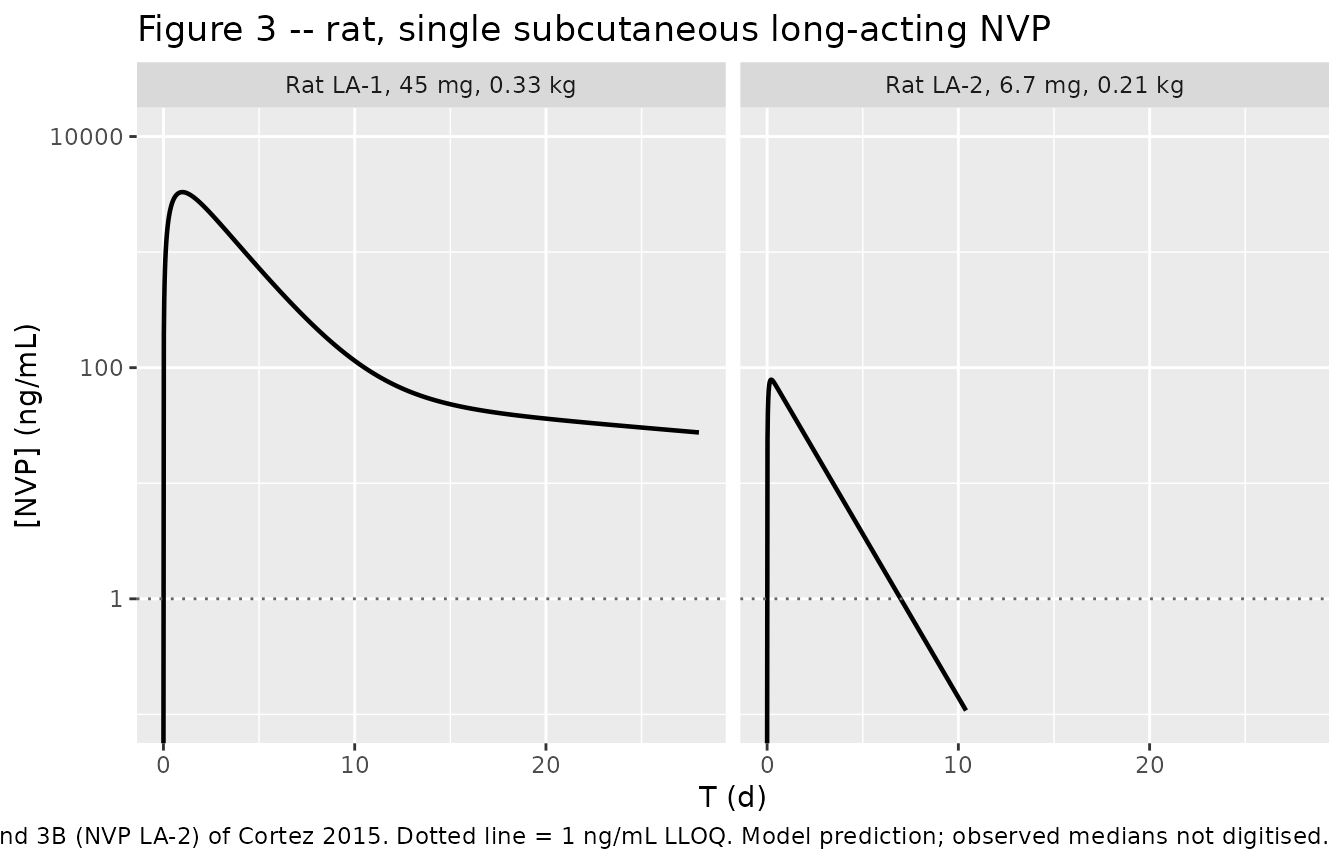

Landmark values read off the published log axes, against the model:

at_day <- function(trt, d) {
  s <- fig3 |> dplyr::filter(treatment == trt)
  s$ng_mL[which.min(abs(s$time - d))]
}

fig3_landmarks <- tibble::tribble(
  ~treatment,                   ~day, ~figure_ng_mL,
  "Rat LA-1, 45 mg, 0.33 kg",      1,          3000,
  "Rat LA-1, 45 mg, 0.33 kg",      6,           500,
  "Rat LA-1, 45 mg, 0.33 kg",     14,            35,
  "Rat LA-1, 45 mg, 0.33 kg",     21,            80,
  "Rat LA-1, 45 mg, 0.33 kg",     28,            50,
  "Rat LA-2, 6.7 mg, 0.21 kg",     1,            70,
  "Rat LA-2, 6.7 mg, 0.21 kg",     3,            50,
  "Rat LA-2, 6.7 mg, 0.21 kg",     7,            40,
  "Rat LA-2, 6.7 mg, 0.21 kg",    14,             3,
  "Rat LA-2, 6.7 mg, 0.21 kg",    21,           1.2
) |>
  dplyr::rowwise() |>
  dplyr::mutate(model_ng_mL = at_day(treatment, day)) |>
  dplyr::ungroup() |>
  dplyr::mutate(ratio = model_ng_mL / figure_ng_mL)

fig3_landmarks |>
  dplyr::transmute("Formulation" = treatment, "Day" = day,
                   "Model (ng/mL)" = signif(model_ng_mL, 3),
                   "Figure 3 (ng/mL)" = figure_ng_mL,
                   "Model / figure" = signif(ratio, 3)) |>
  knitr::kable(caption = "Model versus values digitised from Figure 3.")

Model versus values digitised from Figure 3.
Formulation	Day	Model (ng/mL)	Figure 3 (ng/mL)	Model / figure
Rat LA-1, 45 mg, 0.33 kg	1	3.30e+03	3000.0	1.10e+00
Rat LA-1, 45 mg, 0.33 kg	6	4.76e+02	500.0	9.51e-01
Rat LA-1, 45 mg, 0.33 kg	14	5.34e+01	35.0	1.53e+00
Rat LA-1, 45 mg, 0.33 kg	21	3.49e+01	80.0	4.36e-01
Rat LA-1, 45 mg, 0.33 kg	28	2.75e+01	50.0	5.50e-01
Rat LA-2, 6.7 mg, 0.21 kg	1	4.93e+01	70.0	7.04e-01
Rat LA-2, 6.7 mg, 0.21 kg	3	1.34e+01	50.0	2.68e-01
Rat LA-2, 6.7 mg, 0.21 kg	7	9.90e-01	40.0	2.47e-02
Rat LA-2, 6.7 mg, 0.21 kg	14	1.04e-02	3.0	3.45e-03
Rat LA-2, 6.7 mg, 0.21 kg	21	1.08e-04	1.2	9.04e-05

For NVP LA-1 the model tracks the observed medians through the absorption and early disposition phases, which is what the fit was optimised for (“A modeling approach therefore was adopted that optimized Ka, V, and CL to best fit the observed profiles, with respect to … Cmax … and Tmax”). Beyond day 6 the observed medians scatter either side of the model curve rather than tracking it – the day 14 median falls below it and the day 21 and day 28 medians sit above it. That is expected rather than a transcription problem, and in both directions: the plotted points are medians of at most four animals with SD bars spanning roughly a decade, and BLLOQ values were set to missing rather than imputed, so the late medians are taken over only the animals still quantifiable and are biased upward.

la1 <- fig3_landmarks |> dplyr::filter(grepl("LA-1", treatment), day <= 6)

# Values read by eye off a log axis with 1-decade gridlines; a factor of 2 is
# generous for the digitisation and still breaks instantly on a mis-transcribed
# dose, volume or clearance, which move the curve by an order of magnitude.
stopifnot(all(abs(log(la1$ratio)) < log(2)))

# The paper's abstract: rat plasma NVP was above the 1 ng/mL LLOQ for up to
# 28 days. True for the LA-1 fit.
stopifnot(all(fig3$ng_mL[fig3$time > 0 & grepl("LA-1", fig3$treatment)] > 1))

For NVP LA-2 the model reproduces the peak magnitude but not the sustained tail. This is the consequence of the missing Km, and it is recorded as a known deviation rather than gated:

la2_sim <- fig3 |> dplyr::filter(grepl("LA-2", treatment))
la2 <- fig3_landmarks |> dplyr::filter(grepl("LA-2", treatment))

tibble::tibble(
  quantity = c("Model Cmax (ng/mL)", "Figure 3B peak (ng/mL)",
               "Model / figure at day 7", "Model / figure at day 14"),
  value = c(signif(max(la2_sim$ng_mL), 3), 70,
            signif(la2$ratio[la2$day == 7], 3),
            signif(la2$ratio[la2$day == 14], 3))
)
#> # A tibble: 4 × 2
#>   quantity                    value
#>   <chr>                       <dbl>
#> 1 Model Cmax (ng/mL)       78.7    
#> 2 Figure 3B peak (ng/mL)   70      
#> 3 Model / figure at day 7   0.0247 
#> 4 Model / figure at day 14  0.00345

# GATED: the peak is set by dose / Vc / ka and must be right.
stopifnot(abs(log(max(la2_sim$ng_mL) / 70)) < log(2))

# NOT GATED (known deviation): with elimination reduced to the C << Km limit,
# the profile decays with t1/2 = log(2) * 74 / 48.2 = 1.06 d, so the model
# falls below the observed medians from about day 7 onward. Reproducing that
# tail requires the saturation, i.e. Km, which the paper does not report.
stopifnot(la2$ratio[la2$day == 7] < 0.5)   # observed 0.025: the deviation is real, not noise

Figure 4A and 4B – infant projection, 200 mg NVP LA-1

fig4ab <- sim |>
  dplyr::filter(grepl("Infant LA-1", treatment), time <= 90)

ggplot(fig4ab, aes(time, Cc * 1000)) +
  geom_line(linewidth = 0.8) +
  geom_hline(yintercept = 200,  linetype = "dashed",  colour = "darkred") +
  geom_hline(yintercept = 3000, linetype = "dotdash", colour = "darkorange3") +
  facet_wrap(~treatment) +
  scale_y_log10(limits = c(10, 10000)) +
  labs(x = "Time (d)", y = "[NVP] (ng/mL)",
       title = "Figure 4A / 4B -- infant projection, single 200 mg subcutaneous NVP LA-1",
       caption = paste("Replicates Figure 4A (2.0 kg) and 4B (3.9 kg) of Cortez 2015.",
                       "Dashed = 0.2 ug/mL prophylactic floor;",
                       "dot-dash = 3.0 ug/mL safety ceiling."))
#> Warning in scale_y_log10(limits = c(10, 10000)): log-10 transformation
#> introduced infinite values.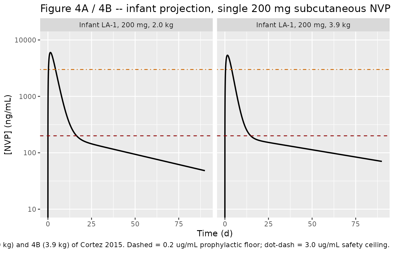

fig4ab_landmarks <- fig4ab |>
  dplyr::group_by(treatment) |>
  dplyr::summarise(
    cmax_ng_mL = max(Cc) * 1000,
    tmax_d     = time[which.max(Cc)],
    d20_ng_mL  = Cc[which.min(abs(time - 20))] * 1000,
    d90_ng_mL  = Cc[which.min(abs(time - 90))] * 1000,
    .groups = "drop"
  )

published_fig4ab <- tibble::tibble(
  treatment  = c("Infant LA-1, 200 mg, 2.0 kg", "Infant LA-1, 200 mg, 3.9 kg"),
  cmax_ng_mL = c(6000, 5000),
  d20_ng_mL  = c( 150,  180),
  d90_ng_mL  = c(  50,   70)
)

cmp4ab <- fig4ab_landmarks |>
  dplyr::select(treatment, cmax_ng_mL, d20_ng_mL, d90_ng_mL) |>
  tidyr::pivot_longer(-treatment, names_to = "landmark", values_to = "model") |>
  dplyr::left_join(
    published_fig4ab |>
      tidyr::pivot_longer(-treatment, names_to = "landmark", values_to = "figure"),
    by = c("treatment", "landmark")
  ) |>
  dplyr::mutate(pct_diff = 100 * (model - figure) / figure)

cmp4ab |>
  dplyr::transmute("Scenario" = treatment, "Landmark" = landmark,
                   "Model (ng/mL)" = signif(model, 3),
                   "Figure 4 (ng/mL)" = figure,
                   "% difference" = round(pct_diff, 1)) |>
  knitr::kable(caption = "Model versus values digitised from Figure 4A and 4B.")

Model versus values digitised from Figure 4A and 4B.
Scenario	Landmark	Model (ng/mL)	Figure 4 (ng/mL)	% difference
Infant LA-1, 200 mg, 2.0 kg	cmax_ng_mL	6000.0	6000	0.0
Infant LA-1, 200 mg, 2.0 kg	d20_ng_mL	165.0	150	9.8
Infant LA-1, 200 mg, 2.0 kg	d90_ng_mL	48.2	50	-3.6
Infant LA-1, 200 mg, 3.9 kg	cmax_ng_mL	5360.0	5000	7.2
Infant LA-1, 200 mg, 3.9 kg	d20_ng_mL	165.0	180	-8.6
Infant LA-1, 200 mg, 3.9 kg	d90_ng_mL	70.4	70	0.5


# Deterministic model versus values read by eye off a 4-decade log axis. 20%
# covers the pixel-level reading error near a gridline; a wrong volume, dose,
# clearance or allometric exponent moves these by 2-10 fold.
stopifnot(max(abs(cmp4ab$pct_diff)) < 20)   # observed 9.8

# The two qualitative claims the paper makes about Figure 4A/B: the heavier
# infant has the higher terminal concentration, and levels fall to "ca.
# 0.2 ug/ml within a few weeks after dosing".
t_cross <- fig4ab |>
  dplyr::group_by(treatment) |>
  dplyr::summarise(t_02_d = min(time[time > 1 & Cc < 0.2]), .groups = "drop")
t_cross
#> # A tibble: 2 × 2
#>   treatment                   t_02_d
#>   <chr>                        <dbl>
#> 1 Infant LA-1, 200 mg, 2.0 kg   16.6
#> 2 Infant LA-1, 200 mg, 3.9 kg   14.8

stopifnot(
  fig4ab_landmarks$d90_ng_mL[2] > fig4ab_landmarks$d90_ng_mL[1],
  all(t_cross$t_02_d > 7), all(t_cross$t_02_d < 35)
)

Figure 4C and 4D – infant projection, 60 mg NVP LA-2

fig4cd <- sim |>
  dplyr::filter(grepl("Infant LA-2", treatment), time <= 90)

ggplot(fig4cd, aes(time, Cc * 1000)) +
  geom_line(linewidth = 0.8) +
  geom_hline(yintercept = 200,  linetype = "dashed",  colour = "darkred") +
  geom_hline(yintercept = 3000, linetype = "dotdash", colour = "darkorange3") +
  facet_wrap(~treatment) +
  scale_y_log10(limits = c(1, 10000)) +
  labs(x = "Time (d)", y = "[NVP] (ng/mL)",
       title = "Figure 4C / 4D -- infant projection, single 60 mg subcutaneous NVP LA-2",
       caption = paste("Attempts Figure 4C (2.0 kg) and 4D (3.9 kg) of Cortez 2015.",
                       "The peak matches; the decay does not -- see the text."))
#> Warning in scale_y_log10(limits = c(1, 10000)): log-10 transformation
#> introduced infinite values.
#> Warning: Removed 18 rows containing missing values or values outside the scale range
#> (`geom_line()`).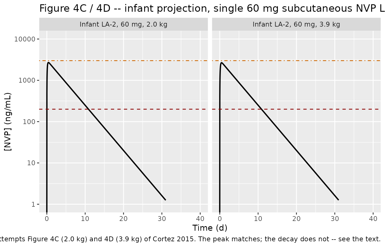

Figure 4C and 4D are plotted as near-straight lines on a log axis, running from about 3,000 ng/mL at t = 0 to about 1,100 ng/mL at day 90. The intercept is exactly 60 mg / 20 L, so V/F = 20 L was clearly used. The slope, however, corresponds to an apparent half-life of roughly 66 days, whereas V/F = 20 L with the CL/F = 0.21 L/h reported in the same Methods paragraph gives 66 hours – the value the paper itself prints two sentences earlier.

fig4cd_check <- fig4cd |>
  dplyr::group_by(treatment) |>
  dplyr::summarise(cmax_ng_mL = max(Cc) * 1000, .groups = "drop") |>
  dplyr::mutate(figure_intercept_ng_mL = 3000,
                pct_diff = 100 * (cmax_ng_mL - figure_intercept_ng_mL) /
                  figure_intercept_ng_mL)
fig4cd_check
#> # A tibble: 2 × 4
#>   treatment                  cmax_ng_mL figure_intercept_ng_mL pct_diff
#>   <chr>                           <dbl>                  <dbl>    <dbl>
#> 1 Infant LA-2, 60 mg, 2.0 kg      2701.                   3000    -9.97
#> 2 Infant LA-2, 60 mg, 3.9 kg      2663.                   3000   -11.2

# Half-life implied by the published panels versus the half-life the published
# systemic parameters give.
implied <- log(2) / (log(2856 / 1136) / 90)      # digitised from Figure 4C
stated  <- log(2) * exp(th("Cortez_2015_nevirapine_human_la2", "lvc")) /
  exp(th("Cortez_2015_nevirapine_human_la2", "lcl"))
tibble::tibble(
  quantity = c("t1/2 implied by Figure 4C (day)",
               "t1/2 from V/F and CL/F as reported (day)",
               "Ratio"),
  value = c(round(implied, 1), round(stated, 2), round(implied / stated, 1))
)
#> # A tibble: 3 × 2
#>   quantity                                 value
#>   <chr>                                    <dbl>
#> 1 t1/2 implied by Figure 4C (day)          67.7 
#> 2 t1/2 from V/F and CL/F as reported (day)  2.75
#> 3 Ratio                                    24.6

# GATED: the peak, which is set by dose / V/F and the rat-derived ka.
stopifnot(all(abs(fig4cd_check$pct_diff) < 15))   # observed -10.0 and -11.2

# NOT GATED (known deviation): the decay. The ratio below is ~24, i.e. very
# close to the 24 h/day that separates 0.21 L/h from 0.21 L/day, which is the
# most economical explanation for the discrepancy. The model encodes the
# parameters as reported in the Methods rather than a reconstruction of the
# figure.
stopifnot(implied / stated > 10)   # observed 24.6

The consequence for the paper’s headline LA-2 claim is direct. With CL/F as reported, a 60 mg dose cannot hold 0.2 ug/mL for 90 days under any absorption profile: maintaining 0.2 ug/mL against a clearance of 5.04 L/day costs about 1 mg/day, so 60 mg is exhausted in roughly 60 days even with perfect zero-order delivery and complete bioavailability.

cl_h   <- exp(th("Cortez_2015_nevirapine_human_la2", "lcl"))   # L/day
target <- 0.2                                                  # ug/mL = mg/L
tibble::tibble(
  quantity = c("Clearance CL/F (L/day)",
               "Dose rate needed to hold 0.2 ug/mL (mg/day)",
               "Maximum days a 60 mg dose can sustain it (upper bound)"),
  value = c(round(cl_h, 2), round(cl_h * target, 3), round(60 / (cl_h * target), 1))
)
#> # A tibble: 3 × 2
#>   quantity                                               value
#>   <chr>                                                  <dbl>
#> 1 Clearance CL/F (L/day)                                  5.04
#> 2 Dose rate needed to hold 0.2 ug/mL (mg/day)             1.01
#> 3 Maximum days a 60 mg dose can sustain it (upper bound) 59.5

# An upper bound from mass balance alone -- no model, no absorption assumption.
stopifnot(60 / (cl_h * target) < 90)

PKNCA validation

sim_nca <- sim |>
  dplyr::filter(!is.na(Cc)) |>
  dplyr::select(id, time, Cc, treatment)

# Guarantee a time = 0 row per subject; pre-dose Cc = 0 is correct for an
# extravascular dose.
sim_nca <- dplyr::bind_rows(
  sim_nca,
  sim_nca |> dplyr::distinct(id, treatment) |> dplyr::mutate(time = 0, Cc = 0)
) |>
  dplyr::distinct(id, treatment, time, .keep_all = TRUE) |>
  dplyr::arrange(id, treatment, time)

conc_obj <- PKNCA::PKNCAconc(sim_nca, Cc ~ time | treatment + id)

dose_df <- events |>
  dplyr::filter(evid == 1L) |>
  dplyr::select(id, time, amt, treatment)
dose_obj <- PKNCA::PKNCAdose(dose_df, amt ~ time | treatment + id)

intervals <- data.frame(
  start = 0, end = Inf,
  cmax = TRUE, tmax = TRUE, aucinf.obs = TRUE, half.life = TRUE
)

nca_res <- PKNCA::pk.nca(PKNCA::PKNCAdata(conc_obj, dose_obj, intervals = intervals))

nca_wide <- as.data.frame(nca_res) |>
  dplyr::select(treatment, PPTESTCD, PPORRES) |>
  tidyr::pivot_wider(names_from = PPTESTCD, values_from = PPORRES)
nca_wide
#> # A tibble: 6 × 15
#>   treatment          cmax  tmax tlast clast.obs lambda.z r.squared adj.r.squared
#>   <chr>             <dbl> <dbl> <dbl>     <dbl>    <dbl>     <dbl>         <dbl>
#> 1 Infant LA-1, 20… 6.00    1.44   450   1.18e-4   0.0168     1.000         1.000
#> 2 Infant LA-1, 20… 5.36    1.48   600   1.65e-4   0.0119     1.000         1.000
#> 3 Infant LA-2, 60… 2.70    0.42    40   1.29e-4   0.252      1.000         1.000
#> 4 Infant LA-2, 60… 2.66    0.48    40   1.30e-4   0.252      1.000         1.000
#> 5 Rat LA-1, 45 mg… 3.30    1      250   2.12e-5   0.0324     1.000         1.000
#> 6 Rat LA-2, 6.7 m… 0.0787  0.22    28   1.14e-9   0.651      1.000         1.000
#> # ℹ 7 more variables: lambda.z.time.first <dbl>, lambda.z.time.last <dbl>,
#> #   lambda.z.n.points <dbl>, clast.pred <dbl>, half.life <dbl>,
#> #   span.ratio <dbl>, aucinf.obs <dbl>

Comparison against analytically derived reference values

Cortez 2015 does not tabulate NCA metrics, so the reference column below is derived analytically from the published parameter estimates rather than transcribed. For a linear model with F = 1 the identities are exact: AUCinf = Dose / (CL/F), and the terminal half-life is log(2)*Vc/CL for the one-compartment fits or log(2)/lambda2 for the two-compartment fits, where lambda2 is the smaller root of the characteristic equation. Cmax and Tmax are taken from the closed form on a fine grid. These are deterministic, so the tolerances are tight.

analytic_reference <- dplyr::bind_rows(lapply(seq_len(nrow(scenarios)), function(i) {
  row <- scenarios[i, ]
  p   <- scaled_params(row$model, row$WT)
  half_life_ref <- if (is.na(p$q)) {
    log(2) * p$vc / p$cl
  } else {
    k10 <- p$cl / p$vc; k12 <- p$q / p$vc; k21 <- p$q / p$vp
    a   <- k10 + k12 + k21
    log(2) / ((a - sqrt(a^2 - 4 * k10 * k21)) / 2)
  }
  tt <- seq(0, min(20, row$t_end), by = 0.0005)
  cc <- analytic_conc(row$model, row$WT, row$amt, tt)
  tibble::tibble(
    treatment      = row$treatment,
    cmax_ref       = max(cc),
    tmax_ref       = tt[which.max(cc)],
    aucinf.obs_ref = row$amt / p$cl,
    half.life_ref  = half_life_ref
  )
}))

cmp_nca <- nca_wide |>
  dplyr::left_join(analytic_reference, by = "treatment") |>
  dplyr::mutate(
    cmax_pct     = 100 * (cmax       - cmax_ref)       / cmax_ref,
    tmax_pct     = 100 * (tmax       - tmax_ref)       / tmax_ref,
    auc_pct      = 100 * (aucinf.obs - aucinf.obs_ref) / aucinf.obs_ref,
    halflife_pct = 100 * (half.life  - half.life_ref)  / half.life_ref
  )

cmp_nca |>
  dplyr::transmute(
    "Scenario"                = treatment,
    "Cmax sim (ug/mL)"        = signif(cmax, 4),
    "Cmax ref (ug/mL)"        = signif(cmax_ref, 4),
    "Tmax sim (d)"            = signif(tmax, 3),
    "Tmax ref (d)"            = signif(tmax_ref, 3),
    "AUCinf sim (ug*d/mL)"    = signif(aucinf.obs, 4),
    "AUCinf ref = Dose/CL"    = signif(aucinf.obs_ref, 4),
    "t1/2 sim (d)"            = signif(half.life, 3),
    "t1/2 ref (d)"            = signif(half.life_ref, 3)
  ) |>
  knitr::kable(
    caption = paste("Simulated NCA versus analytic reference values derived",
                    "from the Cortez 2015 parameter estimates.")
  )

Simulated NCA versus analytic reference values derived from the Cortez 2015 parameter estimates.
Scenario	Cmax sim (ug/mL)	Cmax ref (ug/mL)	Tmax sim (d)	Tmax ref (d)	AUCinf sim (ug*d/mL)	AUCinf ref = Dose/CL	t1/2 sim (d)	t1/2 ref (d)
Infant LA-1, 200 mg, 2.0 kg	6.00200	6.00200	1.44	1.440	39.680	39.680	41.40	41.50
Infant LA-1, 200 mg, 3.9 kg	5.36200	5.36200	1.48	1.480	39.680	39.680	58.20	58.40
Infant LA-2, 60 mg, 2.0 kg	2.70100	2.70100	0.42	0.417	11.900	11.900	2.75	2.75
Infant LA-2, 60 mg, 3.9 kg	2.66300	2.66400	0.48	0.472	11.900	11.900	2.75	2.75
Rat LA-1, 45 mg, 0.33 kg	3.30300	3.30300	1.00	0.991	13.120	13.120	21.40	21.50
Rat LA-2, 6.7 mg, 0.21 kg	0.07872	0.07874	0.22	0.214	0.139	0.139	1.06	1.06


# Deterministic model versus closed-form identity. Cmax and Tmax are limited by
# the 0.02 d observation grid through the peak; AUCinf and half-life by
# lambda-z point selection on the simulated tail.
stopifnot(
  max(abs(cmp_nca$auc_pct))      < 0.3,   # observed 0.035
  max(abs(cmp_nca$cmax_pct))     < 0.2,   # observed 0.015
  max(abs(cmp_nca$tmax_pct))     < 6.0,   # observed 2.6 (grid-limited: 0.02 d on a 0.22 d Tmax)
  max(abs(cmp_nca$halflife_pct)) < 1.0
)

Three structural consequences fall out of that table and are worth stating:

Both LA-1 infant scenarios have the same AUCinf (200 mg / 5.04 L/day = 39.7 ugd/mL), and so do both LA-2 infant scenarios (60 mg / 5.04 L/day = 11.9 ugd/mL), because the human systemic clearance is used at its published value and is not weight-scaled. Only the shape of the profile changes with weight, through the rat-derived parameters.
The projected infant Cmax of ~6 ug/mL for LA-1 exceeds the 3.0 ug/mL steady-state safety ceiling the paper itself nominates, for the first ~4 days after the 200 mg dose. Figures 4A and 4B show the same early excursion above 3 ug/mL, so this is a property of the published simulation rather than of this transcription.
The rat LA-1 apparent terminal half-life (~21 days) is far longer than its absorption half-life (0.367 days), so the study 1 fit is not in flip-flop despite the paper’s general caution about the phenomenon; the sustained exposure comes from the deep peripheral compartment (Vp/F = 14.3 L against Vc/F = 8.66 L with a slow CLp/F of 0.541 L/day).

sim |>
  dplyr::filter(grepl("^Infant", treatment)) |>
  dplyr::group_by(treatment) |>
  dplyr::summarise(
    peak_ug_mL         = round(max(Cc), 2),
    days_above_3_ug_mL = round(ifelse(any(Cc > 3), max(time[Cc > 3]), 0), 2),
    .groups = "drop"
  )
#> # A tibble: 4 × 3
#>   treatment                   peak_ug_mL days_above_3_ug_mL
#>   <chr>                            <dbl>              <dbl>
#> 1 Infant LA-1, 200 mg, 2.0 kg       6                  4.34
#> 2 Infant LA-1, 200 mg, 3.9 kg       5.36               3.9 
#> 3 Infant LA-2, 60 mg, 2.0 kg        2.7                0   
#> 4 Infant LA-2, 60 mg, 3.9 kg        2.66               0

Assumptions and deviations

NVP LA-2 elimination is encoded as first-order at the reported intrinsic clearance. The Discussion describes study 2 as needing saturable elimination, but Table 2 gives only CL/F = 48.2 L/day with footnote d, “Represents intrinsic clearance (Vm/Km), where Vm is the maximal metabolic rate and Km is the Michaelis-Menten constant”. Neither Vm nor Km appears anywhere in the paper, and Vm*C/(Km + C) needs both. Vm/Km is exactly the limiting clearance of that term when C << Km, so the model file uses the published number as a first-order CL/F; nothing is invented and nothing is fitted to the figure. The cost is that the saturation is not represented, and it is visible: the model tracks Figure 3B through roughly day 3 and then falls below the observed medians (the check above records the day 7 and day 14 ratios). This is flagged rather than gated. Recovering the tail would require Km, which is not obtainable from the publication.
Figure 4C and 4D are not reproduced. Those panels start at 60 mg / 20 L = 3.0 ug/mL, confirming the V/F used, but decay with an apparent half-life near 66 days. The V/F = 20 L and CL/F = 0.21 L/h reported in the same Methods paragraph give 66 hours, and the paper prints that t1/2 = 66 h explicitly; the ratio between the figure’s slope and the reported one is close to 24, the number of hours in a day. The model file encodes the parameters as reported rather than a reconstruction of the figure. A mass-balance argument that needs no model is included above: with CL/F = 5.04 L/day, holding 0.2 ug/mL costs ~1 mg/day, so a 60 mg dose cannot sustain the prophylactic floor for the “90 days or longer” the paper claims for LA-2, whatever the release kinetics.
Which human parameters are weight-scaled is inferred, not stated. The Methods say only that the infant systemic parameters “were combined with presystemic rat parameters, essentially the absorption rate constant, ka”, and separately that the allometric exponents are -0.25 / 1 / 0.75. They do not say whether V/F and CL/F were themselves scaled from a reference weight. Reproducing Figure 4A and 4B settles it: the composition encoded here – human Vc/F = 20 L and CL/F = 5.04 L/day used unscaled at both weights, with ka, Vp/F and CLp/F carried from the rat fit and scaled from the 0.33 kg reference – matches the digitised peak, the day-20 value and the day-90 value on both panels. Scaling Vc and CL from any plausible reference weight instead makes the two panels differ in peak height by about two-fold, which the published figure does not show. The same composition is applied to the LA-2 projection for consistency.
CL/F = 0.21 L/h is converted to 5.04 L/day to match this model’s day time base. The paper’s own reported t1/2 of 66 h confirms the conversion (log(2) x 20 L / 0.21 L/h = 66.0 h).
addSd is a unit conversion of the published value. Table 2 reports the study 1 additive residual error as 28.6 ug/liter; the model’s concentration unit is ug/mL (= mg/L), so the encoded value is 0.0286.
Study 2’s residual error is encoded as proportional only. Methods equation 2 allows a combined model but explicitly permits the eps2 = 0 simplification, and Table 2 reports only a proportional term (+/-79.0%) for study 2, with no additive row.
No between-subject variability anywhere, and no residual error on the human models. The rat fits deliberately estimated no BSV (“Due to the low number of rats (n = 4 or n = 10) available for each formulation, no between-subject variability (BSV) was added in the PK model”), and the human projections were naive-pooled mean-concentration simulations with no reported omega or sigma. None is invented here.
Rat volumes and clearances are apparent (/F) and formulation-dependent. The authors are explicit that the absence of an intravenous rat arm means “the values of V and CL derived from the models (Table 2) do not correspond to ‘true’ systemic and peripheral parameters”, and that the estimates for the two formulations “cannot be compared directly”. They are transcribed as published; no attempt is made to reinterpret them as physiological.
The delivered doses, not the nominal doses, are modelled. Study 1’s rat received a nominal 60 mg but the data set assumed 75% delivery (45 mg); study 2’s assumed 80% of 36 mg/kg (6.7 mg). Both are the paper’s own assumptions (Methods, “Population PK data set construction”).
The study 2 column header in Table 2 misprints the formulation as “NVP LA-1”; Methods, Results and the Discussion all identify study 2 with NVP LA-2, and the model file follows them.
Figure landmark values are digitised. The figure_ng_mL columns and the Figure 4 landmark tables were read off the published log-scale plots by eye and are used only as order-of-magnitude gates (a factor of 2 for Figure 3, 20% for Figure 4A/B, 15% for the Figure 4C/D intercept). Every tight assertion in this vignette is against a closed-form identity computed from the published parameter values, not against a digitised point.
The supplement was not obtained. Cortez 2015 cites Figures S1 and S2 in supplemental material as goodness-of-fit diagnostics for the two fits. The ASM supplement endpoint returns HTTP 403, and the EuropePMC supplementary-file service reports “Article with id PMC4291403 is not open access one”; the EuropePMC fullTextXML endpoint returns no supplementary-material element for this article. Nothing in the main text indicates that the supplement holds parameter values beyond Table 2 – it is referenced twice, both times for graphical diagnostics – so the gap does not affect the transcribed parameters. If it turns out to contain Vm and Km, the LA-2 models should be revisited.
The simulation grid extends past the observation windows. Figures are drawn over the published windows (28 days for the rats, 90 days for the infants), but the NCA runs on the same solve extended to roughly ten terminal half-lives per scenario so that aucinf.obs and lambda.z are determined rather than extrapolated from a truncated tail.