Model and source
- Citation: Wu N, Katz DA, An G. Population Target-Mediated Pharmacokinetic/Pharmacodynamic Modeling to Evaluate SPI-62 Exposure and Hepatic 11beta-Hydroxysteroid Dehydrogenase Type 1 (HSD-1) Inhibition in Healthy Adults. Clin Pharmacokinet. 2023;62(9):1275-1288. doi:10.1007/s40262-023-01278-8. PMID:37452998. PMCID:PMC10449972.
- Article: https://doi.org/10.1007/s40262-023-01278-8
- Open-access full text: https://www.ncbi.nlm.nih.gov/pmc/articles/PMC10449972/
- Electronic supplementary material (model-development history Table S1, covariate screening Fig. S2, goodness-of-fit Fig. S3): https://static-content.springer.com/esm/art%3A10.1007%2Fs40262-023-01278-8/MediaObjects/40262_2023_1278_MOESM1_ESM.docx
SPI-62 (formerly ASP3662) is a potent, selective small-molecule inhibitor of 11-beta-hydroxysteroid dehydrogenase type 1 (HSD-1), the enzyme that converts inactive cortisone to active cortisol. It is in clinical development for Cushing’s syndrome, autonomous cortisol secretion, and as adjunctive therapy to prednisolone in polymyalgia rheumatica.
The paper’s central finding is that SPI-62 exhibits
target-mediated drug disposition (TMDD) – a phenomenon usually
associated with biologics, not small molecules. Because SPI-62 binds its
low-capacity target with very high affinity (implied
Kd = Koff / Kon = 0.0272 nM), a low first dose is almost
entirely sequestered on target, so plasma exposure is extraordinarily
low; once the target is saturated by repeated dosing the PK becomes
linear, with accumulation ratios far larger than the elimination
half-life alone could explain. The model links that PK to the
pharmacodynamic readout – hepatic HSD-1 activity, measured as the
urinary ratio of (tetrahydrocortisol + allotetrahydrocortisol) to
tetrahydrocortisone – through a direct inhibitory sigmoid
Imax function.
The structure is:
-
Absorption – a chain of four identical
first-order transit steps
(
depot -> transit1 -> transit2 -> transit3 -> central), all governed by a singleKtr(Eqs. 1-5). The mean transit time is therefore4 / Ktr = 0.45h, which makes the free-concentration peak very sharp (Tmaxaround 0.4 h). -
Disposition – two compartments, linear clearance
CLfromcentraland distribution flowQtoperipheral1(Eqs. 5-6). -
Target binding – explicit second-order association
(
Kon) of the central-compartment concentration to free HSD-1, and first-order dissociation (Koff) of the complex (Eqs. 5, 7). Total targetRtotalis a constant: the paper includes no target synthesis or degradation, so free target isRtotal - complex. -
Pharmacodynamics – hepatic HSD-1 activity as a
percentage of each subject’s own pre-dose baseline (Eq. 8), predicted by
an inhibitory sigmoid
Imaxmodel driven directly by the central-compartment concentration with no effect delay (Eq. 10). Section 3.1 justifies the direct link: there was no time lag between SPI-62Cmaxand maximal HSD-1 inhibition.
#> ℹ parameter labels from comments will be replaced by 'label()'Simultaneous population target-mediated drug disposition (TMDD) PK / PD model for the small-molecule 11-beta-hydroxysteroid dehydrogenase type 1 (HSD-1) inhibitor SPI-62 (formerly ASP3662) in healthy adults (Wu 2023). Oral absorption through a chain of four identical first-order transit steps (depot -> transit1 -> transit2 -> transit3 -> central, all governed by a single Ktr), two-compartment linear disposition (central + peripheral1) with clearance CL and distribution flow Q, and explicit second-order binding of SPI-62 in the central compartment to its pharmacological target HSD-1 (association rate constant Kon, dissociation rate constant Koff) to form a drug-target complex. The total target amount Rtotal is held constant – no target synthesis or degradation is included – so free target is Rtotal minus the complex amount. This saturable, high-affinity / low-capacity binding is what produces SPI-62’s striking nonlinear PK: extremely low plasma exposure after the first low doses (most of the dose is trapped on target), turning into linear PK with unusually high accumulation ratios once the target is saturated by repeated dosing. Hepatic HSD-1 activity, measured as the urinary ratio of (tetrahydrocortisol + allotetrahydrocortisol) to tetrahydrocortisone expressed as a percentage of each subject’s own baseline, is driven directly (no effect delay) by the central-compartment SPI-62 concentration through an inhibitory sigmoid Imax function with half-maximal inhibitory concentration IC50 and power coefficient gamma. Fit by simultaneous PK-PD estimation in NONMEM 7.4.3 (FOCEI, ADVAN13) to pooled data from the SPI-62 first-in-human single-ascending-dose (1-10 mg) and multiple-ascending-dose (0.2-2 mg once daily) phase 1 trials. All PK parameters are apparent (per unit bioavailability) because F is unknown. Exponential inter-individual variability on Vcentral, CL, Ktr, Koff, Rtotal, and IC50; proportional residual error on both the plasma concentration and the HSD-1 activity endpoint. No covariates were retained: age, sex, body weight, and race showed no meaningful relationship with any parameter, so the final model equals the base model. Amounts are carried internally in nmol so that A / V is directly in nmol/L (= nM), the units of Kon, Koff, and IC50; convert an mg dose to nmol by dividing by the SPI-62 molecular weight of 424.4 g/mol and multiplying by 1e6.
Units: doses must be supplied in nmol
This model is unusual in that amounts are carried in nmol,
not mg. Volumes are in L, so A / V is in nmol/L,
which is identical to nM – the unit in which Wu 2023 reports
Kon (nM^-1 h^-1), Koff (h^-1) and
IC50 (nM). Rtotal is an amount in
nmol, matching Table 2. Any dose passed to rxode2::et()
must therefore be converted from mg to nmol first.
The paper does not tabulate a molecular weight, but it states its own
conversion in Sect. 3.3: IC50 = 0.0787 nM
= 0.0334 ng/mL. That pins the molecular weight used
throughout this vignette:
# 0.0334 ng/mL / 0.0787 nM -> g/mol  (Wu 2023 Sect. 3.3)
MW_SPI62 <- 0.0334 / (0.0787e-3)
MW_SPI62
#> [1] 424.3964

mg_to_nmol <- function(mg) mg * 1e6 / MW_SPI62
nmol_to_mg <- function(nmol) nmol * MW_SPI62 * 1e-6
nM_to_ng_mL <- function(nM) nM * MW_SPI62 * 1e-3

# Doses used in the two trials
tibble::tibble(dose_mg = c(0.2, 0.4, 0.7, 1, 2, 3, 6, 10)) |>
  mutate(dose_nmol = round(mg_to_nmol(dose_mg), 1)) |>
  dplyr::rename("Dose (mg)" = dose_mg, "Dose (nmol)" = dose_nmol) |>
knitr::kable(caption = "mg to nmol conversion at MW = 424.4 g/mol.")| Dose (mg) | Dose (nmol) |
|---|---|
| 0.2 | 471.3 |
| 0.4 | 942.5 |
| 0.7 | 1649.4 |
| 1.0 | 2356.3 |
| 2.0 | 4712.6 |
| 3.0 | 7068.9 |
| 6.0 | 14137.7 |
| 10.0 | 23562.9 |
An independent check on that molecular weight: Sect. 3.3 and Sect. 4
both state that the estimated target capacity Rtotal = 5460
nmol “corresponds to approximately 2.2 mg of SPI-62”.
# Rtotal expressed as a mass of SPI-62
round(5460 * MW_SPI62 * 1e-6, 2)  # mg; paper says "approximately 2.2 mg"
#> [1] 2.32
This gives 2.32 mg against the paper’s stated 2.2 mg – a 5% discrepancy that is discussed under Assumptions and deviations below.
Population
The model was fit to pooled data from the two SPI-62 phase 1 trials in 44 healthy adults (Wu 2023 Sect. 2.1, 2.2.1 and Table 1):
- 24 subjects from the single-ascending-dose (SAD) trial – the 1, 3, 6 and 10 mg cohorts (n = 6 active per cohort). The trial also ran 30 and 60 mg cohorts, but those were excluded from this analysis.
- 20 subjects from the low-dose cohorts of the multiple-ascending-dose (MAD) trial – 3 mg loading dose on day 1 then 0.2 mg once daily on days 2-14 (n = 4); 0.4 mg once daily on days 1-14 (n = 4); and 0.7 or 2 mg single dose on day 1 followed by a 6-day washout and then once-daily dosing on days 7-20 (n = 6 each).
The MAD high-dose arms (10, 20 and 50 mg) were deliberately excluded. Sect. 2.1 explains why: including the >= 20 mg groups still converged and gave similar estimates, but degraded the fit at exactly the low doses that are the intended clinical range – and since almost complete hepatic HSD-1 inhibition is achieved at 0.2 mg once daily, the high doses are not informative for dose selection.
Demographics: mean +/- SD age 35.9 +/- 9.65 years, mean +/- SD body weight 76.5 +/- 12.1 kg, 33 males and 11 females, and 26 White / 14 Black / 3 Asian / 1 Native American. Individual minimum-maximum ranges are not tabulated; the distributions appear as histograms in ESM Fig. S1.
The dataset comprised 996 SPI-62 plasma concentrations (222 below the limit of quantification, imputed as LLOQ/2) and 279 baseline-corrected hepatic HSD-1 activity values (one outlier excluded). The LLOQ was 0.1 ng/mL in the SAD trial and 4 pg/mL in the MAD trial.
No covariates are in this model. Sect. 3.2 reports
that exploratory plots of the individual random effects against age,
sex, body weight and race showed no meaningful relationship (p > 0.05
for all plots, ESM Fig. S2), so the formal stepwise covariate search was
never run and the final PK/PD model is identical to the base PK/PD
model. The four screened demographics are recorded in the model’s
covariatesDataExcluded metadata rather than
covariateData, which documents the covariate screen without
implying the model consumes them.
pop <- readModelDb("Wu_2023_SPI_62")()$population
str(pop, max.level = 1)
#> List of 15
#>  $ species       : chr "human"
#>  $ n_subjects    : int 44
#>  $ n_studies     : int 2
#>  $ study_names   : chr [1:2] "SAD -- SPI-62 (ASP3662) first-in-human single ascending dose in healthy adults; 24 of 48 randomised subjects co"| __truncated__ "MAD -- SPI-62 (ASP3662) multiple ascending dose in healthy adults; 20 subjects from the low-dose cohorts only ("| __truncated__
#>  $ age_range     : chr "adults; mean +/- SD 35.9 +/- 9.65 years (individual min-max not tabulated; distribution in ESM Fig. S1)."
#>  $ weight_range  : chr "mean +/- SD 76.5 +/- 12.1 kg (individual min-max not tabulated; distribution in ESM Fig. S1)."
#>  $ sex_female_pct: num 25
#>  $ sex_notes     : chr "33 males and 11 females among the 44 analysis subjects (Wu 2023 Sect. 2.2.1)."
#>  $ race_ethnicity: Named num [1:4] 59.1 31.8 6.8 2.3
#>   ..- attr(*, "names")= chr [1:4] "White" "Black" "Asian" "Native American"
#>  $ race_notes    : chr "Counts as reported in Wu 2023 Sect. 2.2.1: 26 White, 14 Black, 3 Asian, 1 Native American (percentages of 44)."
#>  $ disease_state : chr "Healthy adult volunteers."
#>  $ dose_range    : chr "SAD: 1, 3, 6, and 10 mg single oral dose (the 30 and 60 mg cohorts exist in the trial but were excluded from th"| __truncated__
#>  $ regions       : chr "Not reported."
#>  $ data_records  : chr "996 SPI-62 plasma concentrations (222 below the limit of quantification, imputed as LLOQ/2) and 279 observed ba"| __truncated__
#>  $ notes         : chr "Secondary analysis of the two SPI-62 phase 1 trials; the underlying datasets are proprietary and were not relea"| __truncated__
Source trace
Every ini() value and every model()
equation, with its location in Wu 2023. The same information is recorded
as an in-file comment beside each entry in
inst/modeldb/specificDrugs/Wu_2023_SPI_62.R.
| Equation / parameter | Value | Source location |
|---|---|---|
d/dt(depot) |
n/a | Eq. 1, p. 1278 (-Ktr * A_depot; initial condition
Dose * F) |
d/dt(transit1) |
n/a | Eq. 2, p. 1278 |
d/dt(transit2) |
n/a | Eq. 3, p. 1278 |
d/dt(transit3) |
n/a | Eq. 4, p. 1278 |
d/dt(central) |
n/a | Eq. 5, p. 1278 (transit input, Kon/Koff
binding, CL/Vcen, Q exchange) |
d/dt(peripheral1) |
n/a | Eq. 6, p. 1278 |
d/dt(complex) |
n/a | Eq. 7, p. 1279
(Kon * Ccen * (Rtotal - RC) - Koff * RC) |
| Baseline correction of the PD observation | n/a | Eq. 8, p. 1279 (activity as % of each subject’s own baseline) |
| HSD-1 inhibition (%) = 100 - activity | n/a | Eq. 9, p. 1279 |
hsd1activity (sigmoid Imax) |
n/a | Eq. 10, p. 1279; final form confirmed as ESM Table S1 row “13-final” |
lktr (Ktr) |
8.82 1/h | Table 2 (RSE 11%) |
lcl (CL/F) |
10.1 L/h | Table 2 (RSE 6%); apparent, Table 2 footnote a |
lvc (Vcen/F) |
152 L | Table 2 (RSE 16%); apparent, Table 2 footnote a |
lq (Q/F) |
2.38 L/h | Table 2 (RSE 12%); apparent, Table 2 footnote a |
lvp (Vperi/F) |
116 L | Table 2 (RSE 6%); apparent, Table 2 footnote a |
lfdepot (F) |
fixed at 1 | Eq. 1 and Table 2 footnote a (F unknown; only apparent parameters estimated) |
lkon (Kon) |
8.43 1/(nM*h) | Table 2 (RSE 6%) |
lkoff (Koff) |
0.229 1/h | Table 2 (RSE 31%) |
lrtot (Rtotal) |
5460 nmol | Table 2 (RSE 7%) |
limax (Imax) |
99.9% -> 0.999 | Table 2 (RSE 2%), stored as the fraction Eq. 10 consumes |
lec50 (IC50) |
0.0787 nM | Table 2 (RSE 16%) |
lhill (gamma) |
0.441 | Table 2 (RSE 7%) |
etalvc |
0.238514 | Table 2 IIV Vcentral 51.9% (RSE 33%, shrinkage 14%);
omega^2 = log(CV^2 + 1)
|
etalcl |
0.036201 | Table 2 IIV CL 19.2% (RSE 84%, shrinkage 21%) |
etalktr |
0.224745 | Table 2 IIV Ktr 50.2% (RSE 38%, shrinkage 7%) |
etalkoff |
0.882155 | Table 2 IIV Koff 119% (RSE 55%, shrinkage 15%) |
etalrtot |
0.072902 | Table 2 IIV Rtotal 27.5% (RSE 31%, shrinkage 9%) |
etalec50 |
0.144987 | Table 2 IIV IC50 39.5% (RSE 63%, shrinkage 37%) |
propSd |
0.274 | Table 2 sigma_PK 27.4% (RSE 3%, shrinkage 7%) |
propSd_hsd1activity |
0.193 | Table 2 sigma_PD 19.3% (RSE 12%, shrinkage 5%) |
| MW = 424.4 g/mol (unit conversion only, not a model parameter) | 424.4 | Derived from Sect. 3.3
IC50 = 0.0787 nM = 0.0334 ng/mL
|
The implied dissociation equilibrium constant is a useful cross-check on the two binding parameters:
# Kd = Koff / Kon; paper Sect. 3.3 reports 0.0272 nM, Sect. 4 reports 27.2 pM
round(0.229 / 8.43, 4)
#> [1] 0.0272
Virtual cohort
The original trial data are proprietary and were not released (the
paper’s data availability statement is explicit about this), so the
figures below use virtual cohorts dosed on the published regimens. The
model carries no covariates, so a virtual cohort needs
no demographic sampling at all – only the dosing regimen and observation
schedule. Between-subject variability comes entirely from the six
eta terms.
Cohorts are 100 subjects per arm (the paper simulated 1000 per arm for Figs. 7-8; 100 is ample for the percentile ribbons here and keeps the vignette inside its render budget).
Two event-table details matter for this model:
-
Observation rows must carry
dvid. The model has two endpoints (Cc ~ prop(...)andhsd1activity ~ prop(...)), so rxode2 needs each observation row assigned to an endpoint.cmt = "central"alone raises'dvid'->'cmt' or 'cmt' on observation record ... undefined compartment. Settingcmt = "central"(the ODE state) together withdvid = 1Lresolves it, and rxode2 still returns bothCcandhsd1activityas columns on every observation row – so one set of observation rows is enough for both endpoints. - Doses are in nmol (see above).
N_PER_ARM <- 100L

# Build one arm. `doses` is a data frame of (time, mg, ii, addl) dosing records,
# so a loading dose followed by a maintenance regimen is expressible in one arm.
make_arm <- function(n, arm, doses, tobs, id_offset = 0L) {
  ids <- id_offset + seq_len(n)
  dose_rows <- doses |>
    dplyr::rowwise() |>
    dplyr::reframe(
      id   = ids,
      time = time,
      amt  = mg_to_nmol(mg),
      evid = 1L,
      cmt  = "depot",
      dvid = NA_integer_,
      ii   = ii,
      addl = addl
    )
  obs_rows <- tidyr::expand_grid(id = ids, time = tobs) |>
    dplyr::mutate(
      amt = NA_real_, evid = 0L, cmt = "central", dvid = 1L, ii = 0, addl = 0L
    )
  dplyr::bind_rows(dose_rows, obs_rows) |>
    dplyr::mutate(arm = arm) |>
    dplyr::arrange(id, time, dplyr::desc(evid))
}

# One dosing record helper
dose_rec <- function(time, mg, ii = 0, addl = 0L) {
  tibble::tibble(time = time, mg = mg, ii = ii, addl = addl)
}

solve_arms <- function(events) {
  rxode2::rxSolve(
    readModelDb("Wu_2023_SPI_62"), events,
    keep  = "arm",
    # Concentrations of interest are in the pg/mL range, so solve tightly.
    atol = 1e-12, rtol = 1e-10
  ) |>
    as.data.frame()
}
Replicate published figures
Figures 4 and 5 – observed regimens (SAD and MAD)
The SAD arms are single oral doses of 1, 3, 6 and 10 mg. Sampling
follows Table 1, plus a fine early grid so the sharp Tmax
near 0.4 h is resolved.
set.seed(20230715)

t_sad <- sort(unique(c(seq(0, 6, by = 0.1), c(0.5, 1, 1.5, 2, 3, 4, 6, 8, 10, 12,
                                             18, 24, 36, 48, 72, 96, 120))))
sad_doses <- c(1, 3, 6, 10)

events_sad <- dplyr::bind_rows(
  lapply(seq_along(sad_doses), function(i) {
    make_arm(
      N_PER_ARM,
      arm = sprintf("%g mg single dose", sad_doses[i]),
      doses = dose_rec(0, sad_doses[i]),
      tobs = t_sad,
      id_offset = (i - 1L) * N_PER_ARM
    )
  })
)
stopifnot(!anyDuplicated(unique(events_sad[, c("id", "time", "evid")])))

sim_sad <- solve_arms(events_sad)
#> ℹ parameter labels from comments will be replaced by 'label()'
sim_sad |>
  mutate(arm = factor(arm, levels = sprintf("%g mg single dose", sad_doses))) |>
  group_by(arm, time) |>
  summarise(
    Q05 = quantile(nM_to_ng_mL(Cc), 0.05),
    Q50 = quantile(nM_to_ng_mL(Cc), 0.50),
    Q95 = quantile(nM_to_ng_mL(Cc), 0.95),
    .groups = "drop"
  ) |>
  filter(Q50 > 0) |>
  ggplot(aes(time, Q50)) +
  geom_ribbon(aes(ymin = Q05, ymax = Q95), alpha = 0.25) +
  geom_line() +
  facet_wrap(~arm, scales = "free_y") +
  scale_x_continuous(limits = c(0, 120)) +
  labs(
    x = "Time (h)", y = "SPI-62 plasma concentration (ng/mL)",
    title = "Figure 4 (single-dose arms) -- SPI-62 plasma concentration",
    caption = "Median with 5th-95th percentile ribbon, 100 virtual subjects per arm."
  )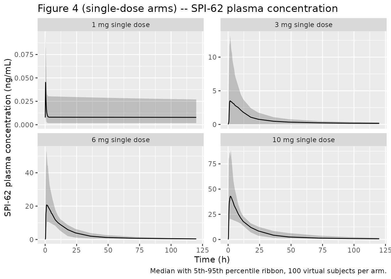
Replicates the single-dose panels of Figure 4 of Wu 2023.
The MAD low-dose arms reproduce the published regimens exactly, including the 3 mg loading dose in the 0.2 mg arm and the 6-day washout in the 0.7 and 2 mg arms.
set.seed(20230716)

t_mad <- sort(unique(c(seq(0, 6, by = 0.25), seq(0, 24 * 27, by = 2))))

events_mad <- dplyr::bind_rows(
  # 3 mg loading dose day 1, then 0.2 mg QD days 2-14
  make_arm(N_PER_ARM, "0.2 mg QD (3 mg loading dose)",
           dplyr::bind_rows(dose_rec(0, 3),
                            dose_rec(24, 0.2, ii = 24, addl = 12L)),
           t_mad, id_offset = 0L),
  # 0.4 mg QD days 1-14
  make_arm(N_PER_ARM, "0.4 mg QD (days 1-14)",
           dose_rec(0, 0.4, ii = 24, addl = 13L),
           t_mad, id_offset = 1L * N_PER_ARM),
  # 0.7 mg single dose day 1, 6-day washout, QD days 7-20
  make_arm(N_PER_ARM, "0.7 mg SD + QD (days 7-20)",
           dplyr::bind_rows(dose_rec(0, 0.7),
                            dose_rec(24 * 6, 0.7, ii = 24, addl = 13L)),
           t_mad, id_offset = 2L * N_PER_ARM),
  # 2 mg single dose day 1, 6-day washout, QD days 7-20
  make_arm(N_PER_ARM, "2 mg SD + QD (days 7-20)",
           dplyr::bind_rows(dose_rec(0, 2),
                            dose_rec(24 * 6, 2, ii = 24, addl = 13L)),
           t_mad, id_offset = 3L * N_PER_ARM)
)
stopifnot(!anyDuplicated(unique(events_mad[, c("id", "time", "evid")])))

sim_mad <- solve_arms(events_mad)

mad_levels <- c("0.2 mg QD (3 mg loading dose)", "0.4 mg QD (days 1-14)",
                "0.7 mg SD + QD (days 7-20)", "2 mg SD + QD (days 7-20)")
sim_mad |>
  mutate(arm = factor(arm, levels = mad_levels)) |>
  group_by(arm, time) |>
  summarise(
    conc = median(nM_to_ng_mL(Cc)),
    act  = median(hsd1activity),
    .groups = "drop"
  ) |>
  tidyr::pivot_longer(c(conc, act), names_to = "endpoint", values_to = "value") |>
  mutate(endpoint = factor(
    endpoint, levels = c("conc", "act"),
    labels = c("SPI-62 (ng/mL)", "Hepatic HSD-1 activity (% of baseline)")
  )) |>
  ggplot(aes(time / 24, value)) +
  geom_line() +
  facet_grid(endpoint ~ arm, scales = "free_y") +
  labs(
    x = "Time (days)", y = NULL,
    title = "Figure 5 -- SPI-62 concentration and hepatic HSD-1 activity",
    caption = "Median of 100 virtual subjects per arm."
  ) +
  theme(strip.text.x = element_text(size = 7))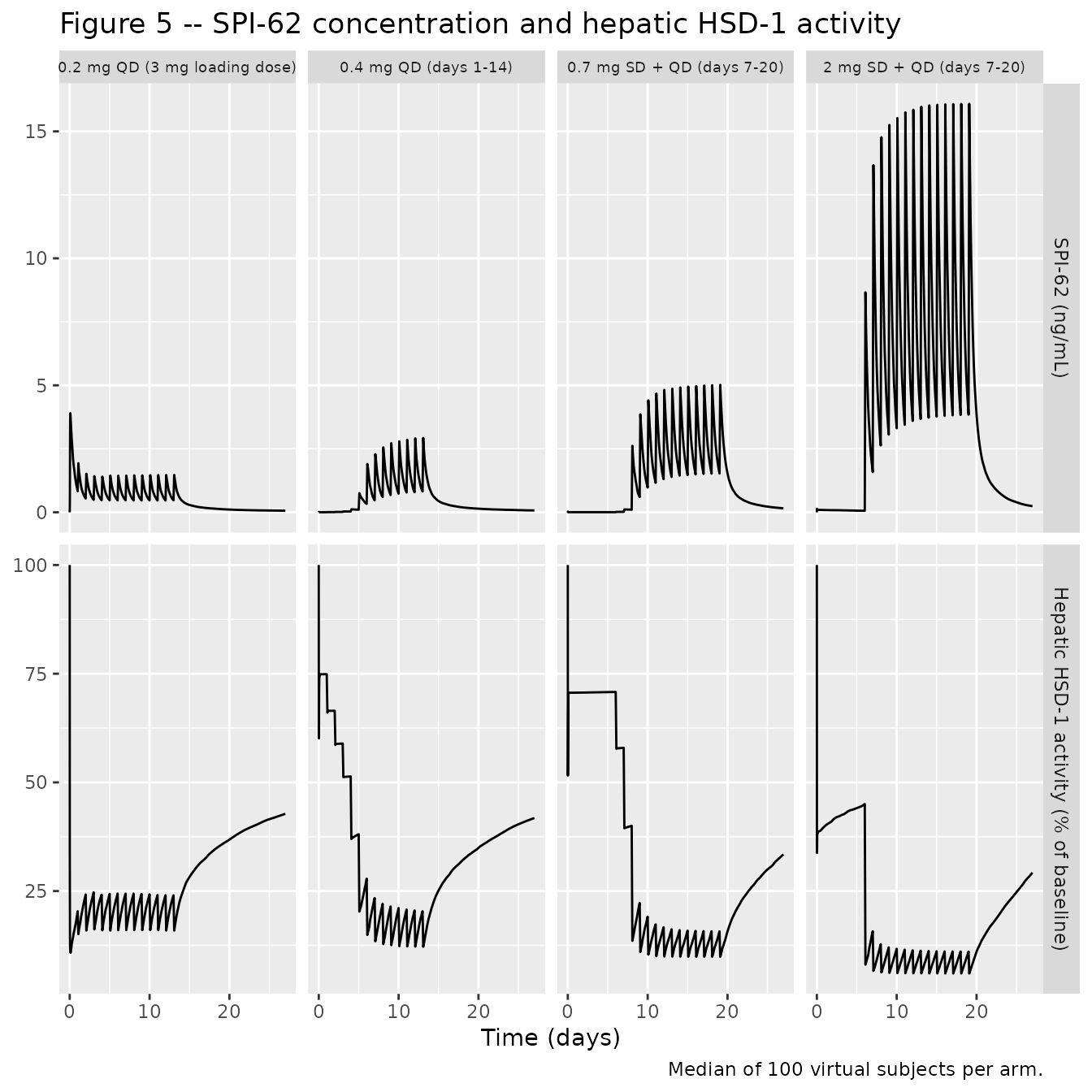
Replicates Figure 5 of Wu 2023: SPI-62 concentration and hepatic HSD-1 activity after 0.2, 0.4, 0.7 and 2 mg once-daily dosing.
Two behaviours the paper highlights are visible here. First, hepatic HSD-1 activity is driven far down even at 0.2-0.4 mg, doses at which plasma concentrations are in the low pg/mL range. Second, the PD effect long outlasts dosing – activity has still not returned to baseline a week after the last dose.
Figure 1 – inhibition is substantial from the first low dose
sim_mad |>
  mutate(arm = factor(arm, levels = mad_levels)) |>
  group_by(arm, time) |>
  summarise(inhibition = median(100 - hsd1activity), .groups = "drop") |>
  ggplot(aes(time / 24, inhibition, colour = arm)) +
  geom_line(linewidth = 0.7) +
  scale_y_continuous(limits = c(0, 100)) +
  labs(
    x = "Time (days)", y = "Hepatic HSD-1 inhibition (%)",
    colour = "Regimen",
    title = "Figure 1 -- hepatic HSD-1 inhibition over time",
    caption = "Median of 100 virtual subjects per arm. Inhibition (%) = 100 - activity (Eq. 9)."
  ) +
  theme(legend.position = "bottom", legend.direction = "vertical")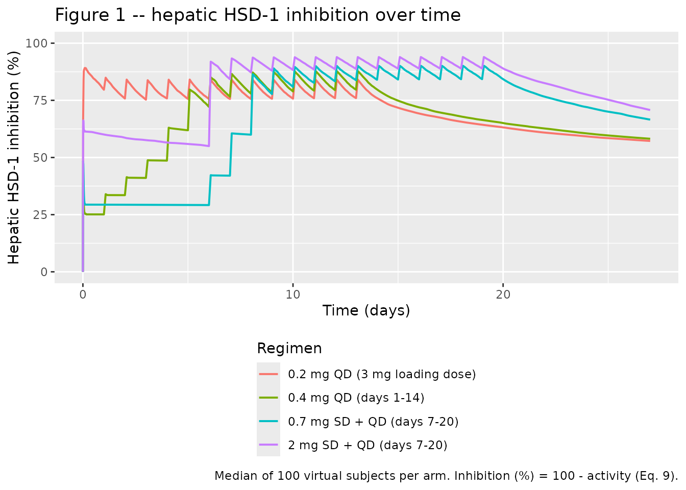
Replicates Figure 1 of Wu 2023: hepatic HSD-1 inhibition alongside model-predicted SPI-62 concentration.
The paper reports two specific quantitative anchors for the 0.7 mg
single dose (Sect. 4): more than 40% hepatic HSD-1 inhibition at a mean
Cmax of only about 0.02 ng/mL, and more than 30% inhibition
still present on day 6 of the washout. Both are reproduced:
sim_mad |>
  filter(arm == "0.7 mg SD + QD (days 7-20)", time <= 24 * 6) |>
  group_by(id) |>
  summarise(max_inhibition = max(100 - hsd1activity), .groups = "drop") |>
  summarise(
    `Mean maximal inhibition, 0.7 mg single dose (%)` = round(mean(max_inhibition), 1)
  ) |>
knitr::kable(caption = "Paper Sect. 4: 'more than 40% of hepatic HSD-1 inhibition'.")| Mean maximal inhibition, 0.7 mg single dose (%) |
|---|
| 50.8 |
sim_mad |>
  filter(arm == "0.7 mg SD + QD (days 7-20)", time == 24 * 6) |>
  summarise(
    `Mean inhibition at day 6 of washout (%)` = round(mean(100 - hsd1activity), 1)
  ) |>
knitr::kable(caption = "Paper Sect. 4: '> 30% inhibition being observed on day 6'.")| Mean inhibition at day 6 of washout (%) |
|---|
| 30.8 |
Figure 2 – the exposure-response relationship
Figure 2 of the paper is a log-scale scatter of observed
baseline-corrected HSD-1 activity against time-matched model-predicted
SPI-62 concentration. Overlaying the analytical Imax curve
on the simulated points shows that the scatter is exactly Eq. 10 plus
residual variability in IC50.
imax_curve <- tibble::tibble(Cc = 10^seq(-4, 2, length.out = 400)) |>
  mutate(activity = 100 * (1 - 0.999 * Cc^0.441 / (0.0787^0.441 + Cc^0.441)))

sim_mad |>
  filter(!is.na(Cc), Cc > 0) |>
  slice_sample(n = 4000) |>
  ggplot(aes(Cc, hsd1activity)) +
  geom_point(alpha = 0.12, size = 0.7) +
  geom_line(data = imax_curve, aes(Cc, activity), colour = "red", linewidth = 0.9) +
  scale_x_log10() +
  geom_vline(xintercept = 0.0787, linetype = "dashed") +
  labs(
    x = "SPI-62 plasma concentration (nM, log scale)",
    y = "Hepatic HSD-1 activity (% of baseline)",
    title = "Figure 2 -- exposure-response for hepatic HSD-1 inhibition",
    caption = paste("Points: 4000 sampled simulated observations from the MAD arms.",
                    "Red line: Eq. 10 at typical values.",
                    "Dashed line: IC50 = 0.0787 nM.")
  )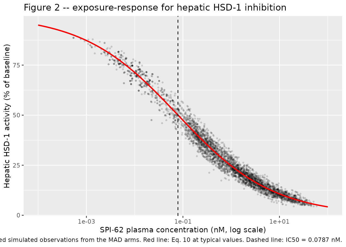
Replicates Figure 2 of Wu 2023: hepatic HSD-1 activity versus time-matched SPI-62 concentration, with the Eq. 10 typical-value curve overlaid.
Target-mediated nonlinearity
The defining PK feature of this model is that dose-normalised
exposure rises steeply with dose over the range in which the target is
being saturated, then flattens. The paper ties the transition to
Rtotal: 5460 nmol “corresponds to approximately 2.2 mg of
SPI-62, which comports well with the dose range in which PK nonlinearity
is prominent” (Sect. 3.3, Sect. 4).
dose_grid <- c(0.2, 0.4, 0.7, 1, 1.5, 2, 3, 4, 6, 10, 20, 30)

auc_by_dose <- lapply(dose_grid, function(d) {
  ev <- make_arm(1L, sprintf("%g mg", d), dose_rec(0, d), seq(0, 72, by = 0.2))
  s <- rxode2::rxSolve(readModelDb("Wu_2023_SPI_62"), ev,
                       omega = NA, sigma = NA, atol = 1e-12, rtol = 1e-10) |>
    as.data.frame()
  tibble::tibble(
    dose_mg = d,
    auc = sum(diff(s$time) * (head(s$Cc, -1) + tail(s$Cc, -1)) / 2)
  )
}) |>
  dplyr::bind_rows() |>
  mutate(auc_per_mg = auc / dose_mg)

ggplot(auc_by_dose, aes(dose_mg, auc_per_mg)) +
  geom_line() +
  geom_point() +
  geom_vline(xintercept = 5460 * MW_SPI62 * 1e-6, linetype = "dashed", colour = "red") +
  scale_x_log10() +
  scale_y_log10() +
  labs(
    x = "Single dose (mg, log scale)",
    y = "Dose-normalised AUC(0-72 h) (nM*h per mg, log scale)",
    title = "Target-mediated nonlinearity in SPI-62 exposure",
    caption = "Typical-value simulation. Red dashed line: Rtotal expressed as mass of SPI-62 (2.32 mg)."
  )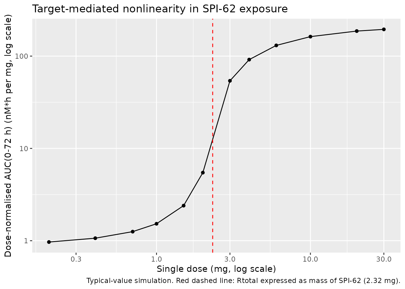
Dose-normalised single-dose AUC(0-72 h) at typical parameter values. The steep rise flattens once the dose exceeds the target capacity Rtotal (5460 nmol, about 2.3 mg).
Dose-normalised AUC increases by more than two orders of magnitude
between 0.7 mg and 30 mg, with the inflection sitting on the
Rtotal line – the paper’s mechanistic claim, reproduced
from the packaged parameters.
Figure 7 – simulated once-daily regimens
set.seed(20230717)

fig7_doses <- c(0.4, 1, 2, 3, 6, 10)
t_fig7 <- sort(unique(c(seq(0, 6, by = 0.25), seq(0, 24 * 21, by = 2))))

events_fig7 <- dplyr::bind_rows(
  lapply(seq_along(fig7_doses), function(i) {
    make_arm(
      N_PER_ARM,
      arm = sprintf("%g mg QD", fig7_doses[i]),
      doses = dose_rec(0, fig7_doses[i], ii = 24, addl = 13L),
      tobs = t_fig7,
      id_offset = (i - 1L) * N_PER_ARM
    )
  })
)
stopifnot(!anyDuplicated(unique(events_fig7[, c("id", "time", "evid")])))

sim_fig7 <- solve_arms(events_fig7)
sim_fig7 |>
  mutate(arm = factor(arm, levels = sprintf("%g mg QD", fig7_doses))) |>
  group_by(arm, time) |>
  summarise(
    conc_Q05 = quantile(nM_to_ng_mL(Cc), 0.05),
    conc_Q50 = quantile(nM_to_ng_mL(Cc), 0.50),
    conc_Q95 = quantile(nM_to_ng_mL(Cc), 0.95),
    act_Q05  = quantile(hsd1activity, 0.05),
    act_Q50  = quantile(hsd1activity, 0.50),
    act_Q95  = quantile(hsd1activity, 0.95),
    .groups = "drop"
  ) |>
  tidyr::pivot_longer(
    -c(arm, time),
    names_to = c("endpoint", "stat"), names_sep = "_"
  ) |>
  tidyr::pivot_wider(names_from = stat, values_from = value) |>
  mutate(endpoint = factor(
    endpoint, levels = c("conc", "act"),
    labels = c("SPI-62 (ng/mL)", "Hepatic HSD-1 activity (% of baseline)")
  )) |>
  ggplot(aes(time / 24, Q50)) +
  geom_ribbon(aes(ymin = Q05, ymax = Q95), alpha = 0.25) +
  geom_line() +
  facet_grid(endpoint ~ arm, scales = "free_y") +
  labs(
    x = "Time (days)", y = NULL,
    title = "Figure 7 -- simulated once-daily regimens, days 1-14",
    caption = "Median with 5th-95th percentile ribbon, 100 virtual subjects per arm."
  ) +
  theme(strip.text.x = element_text(size = 7))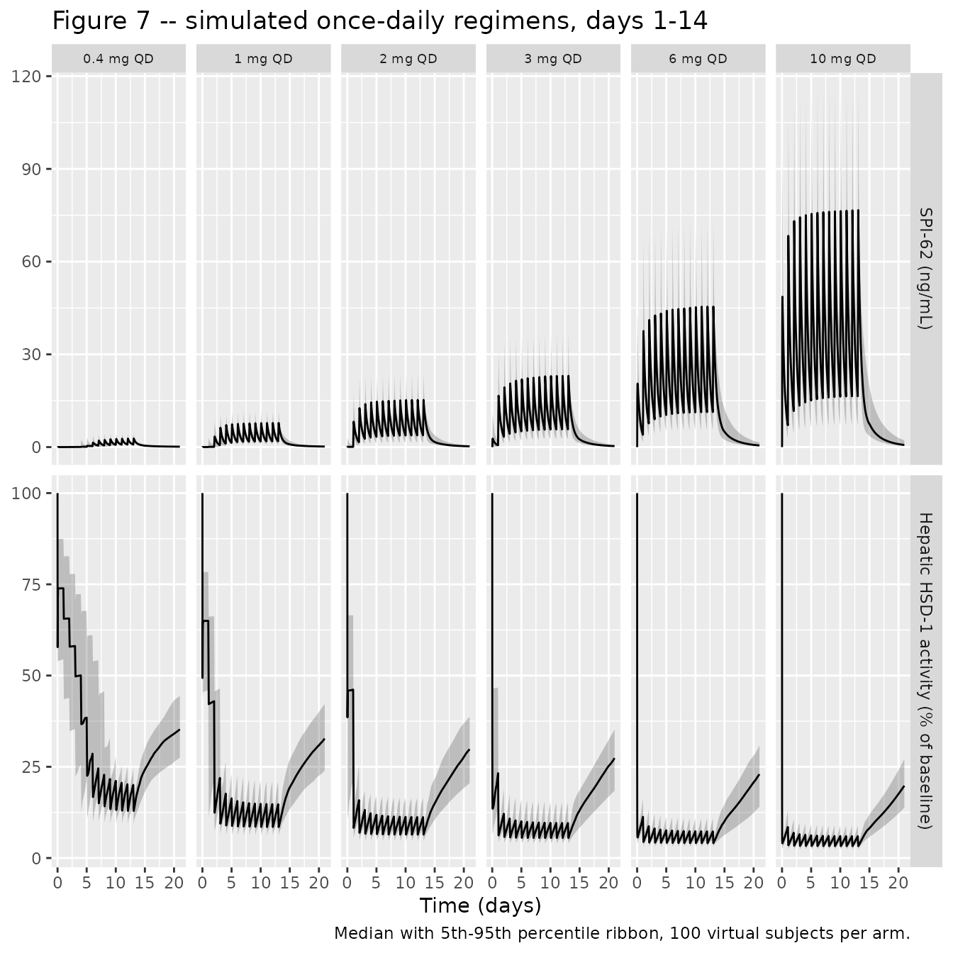
Replicates Figure 7 of Wu 2023: median with 5th-95th percentiles of simulated SPI-62 concentration and hepatic HSD-1 activity for 0.4-10 mg once daily on days 1-14.
The paper draws three conclusions from its Figure 7 (Sect. 3.5, Sect. 4): full inhibition once the dose is at least 2 mg once daily; a dose-dependent time to maximal effect (about 10 days at 0.4 mg once daily, versus about 1-2 days at the higher doses); and variability in simulated HSD-1 activity that shrinks as dose rises. All three are reproduced:
trough_summary <- sim_fig7 |>
  filter(time %in% (24 * seq_len(14))) |>
  group_by(arm, day = time / 24) |>
  summarise(
    inhibition = median(100 - hsd1activity),
    iqr_activity = IQR(hsd1activity),
    .groups = "drop"
  )

trough_summary |>
  group_by(arm) |>
  summarise(
    `Day-14 trough inhibition (%)` = round(inhibition[day == 14], 1),
    `Day reaching 95% of day-14 effect` = day[which(inhibition >= 0.95 * inhibition[day == 14])[1]],
    `IQR of activity at day 14 (% points)` = round(iqr_activity[day == 14], 2),
    .groups = "drop"
  ) |>
  mutate(dose = as.numeric(sub(" mg QD", "", arm))) |>
  arrange(dose) |>
  select(-dose) |>
  dplyr::rename(Regimen = arm) |>
  knitr::kable(caption = paste(
    "Dose-dependence of the magnitude and onset of hepatic HSD-1 inhibition,",
    "and the narrowing of variability with dose (Wu 2023 Sect. 3.5)."
))| Regimen | Day-14 trough inhibition (%) | Day reaching 95% of day-14 effect | IQR of activity at day 14 (% points) |
|---|---|---|---|
| 0.4 mg QD | 80.1 | 8 | 4.11 |
| 1 mg QD | 85.3 | 4 | 4.38 |
| 2 mg QD | 88.8 | 3 | 3.27 |
| 3 mg QD | 90.4 | 2 | 2.67 |
| 6 mg QD | 92.7 | 1 | 2.14 |
| 10 mg QD | 94.0 | 1 | 2.01 |
Persistence after the last dose (paper: “substantial inhibition through 7 days after the last dose”):
sim_fig7 |>
  filter(time == 24 * 20) |>
  group_by(arm) |>
  summarise(inhibition = round(median(100 - hsd1activity), 1), .groups = "drop") |>
  mutate(dose = as.numeric(sub(" mg QD", "", arm))) |>
  arrange(dose) |>
  select(-dose) |>
  dplyr::rename(Regimen = arm, `Inhibition 7 days after last dose (%)` = inhibition) |>
knitr::kable(caption = "Wu 2023 Sect. 3.5: the inhibitory effect is long lasting.")| Regimen | Inhibition 7 days after last dose (%) |
|---|---|
| 0.4 mg QD | 66.0 |
| 1 mg QD | 69.1 |
| 2 mg QD | 72.3 |
| 3 mg QD | 74.8 |
| 6 mg QD | 79.3 |
| 10 mg QD | 82.4 |
Figure 8 – loading dose
set.seed(20230718)

events_fig8 <- dplyr::bind_rows(
  make_arm(N_PER_ARM, "3 mg load, then 0.4 mg QD",
           dplyr::bind_rows(dose_rec(0, 3), dose_rec(24, 0.4, ii = 24, addl = 12L)),
           t_fig7, id_offset = 0L),
  make_arm(N_PER_ARM, "3 mg load, then 1 mg QD",
           dplyr::bind_rows(dose_rec(0, 3), dose_rec(24, 1, ii = 24, addl = 12L)),
           t_fig7, id_offset = N_PER_ARM)
)
stopifnot(!anyDuplicated(unique(events_fig8[, c("id", "time", "evid")])))

sim_fig8 <- solve_arms(events_fig8)
sim_fig8 |>
  group_by(arm, time) |>
  summarise(
    conc_Q05 = quantile(nM_to_ng_mL(Cc), 0.05),
    conc_Q50 = quantile(nM_to_ng_mL(Cc), 0.50),
    conc_Q95 = quantile(nM_to_ng_mL(Cc), 0.95),
    act_Q05  = quantile(hsd1activity, 0.05),
    act_Q50  = quantile(hsd1activity, 0.50),
    act_Q95  = quantile(hsd1activity, 0.95),
    .groups = "drop"
  ) |>
  tidyr::pivot_longer(-c(arm, time), names_to = c("endpoint", "stat"), names_sep = "_") |>
  tidyr::pivot_wider(names_from = stat, values_from = value) |>
  mutate(endpoint = factor(
    endpoint, levels = c("conc", "act"),
    labels = c("SPI-62 (ng/mL)", "Hepatic HSD-1 activity (% of baseline)")
  )) |>
  ggplot(aes(time / 24, Q50)) +
  geom_ribbon(aes(ymin = Q05, ymax = Q95), alpha = 0.25) +
  geom_line() +
  facet_grid(endpoint ~ arm, scales = "free_y") +
  labs(
    x = "Time (days)", y = NULL,
    title = "Figure 8 -- loading dose followed by once-daily maintenance",
    caption = "Median with 5th-95th percentile ribbon, 100 virtual subjects per arm."
  )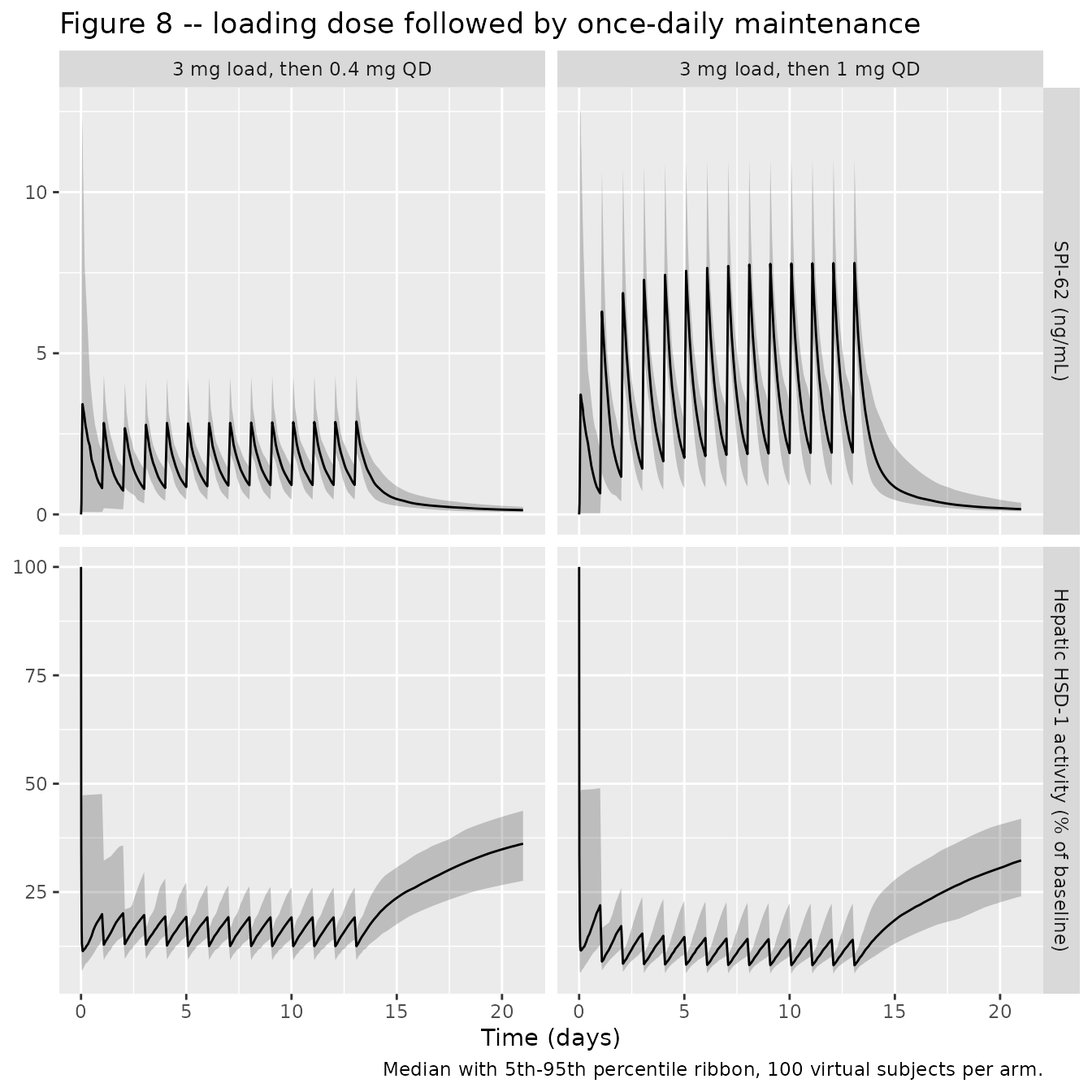
Replicates Figure 8 of Wu 2023: a 3 mg loading dose on day 1 followed by 0.4 mg or 1 mg once daily on days 2-14.
The paper’s point about Figure 8 is that a loading dose “could bring HSD-1 inhibition to its maximum level within the first dose interval”. Comparing the day-1 inhibition with and without the 3 mg loading dose confirms it:
dplyr::bind_rows(
  sim_fig8 |> filter(time == 24) |> mutate(regimen = arm),
  sim_fig7 |> filter(time == 24, arm %in% c("0.4 mg QD", "1 mg QD")) |>
    mutate(regimen = paste0(arm, " (no loading dose)"))
) |>
  group_by(regimen) |>
  summarise(inhibition = round(median(100 - hsd1activity), 1), .groups = "drop") |>
  dplyr::rename(Regimen = regimen, `Inhibition at 24 h (%)` = inhibition) |>
knitr::kable(caption = "A 3 mg loading dose reaches near-maximal inhibition within the first dose interval.")| Regimen | Inhibition at 24 h (%) |
|---|---|
| 0.4 mg QD (no loading dose) | 26.1 |
| 1 mg QD (no loading dose) | 35.0 |
| 3 mg load, then 0.4 mg QD | 80.1 |
| 3 mg load, then 1 mg QD | 78.1 |
PKNCA validation
Wu 2023 does not publish an NCA table, but it does report one
NCA-style value: the mean Cmax of a single 0.7 mg dose was
0.0185 ng/mL (Sect. 3.3; “only 0.02 ng/mL” in Sect. 4). NCA is run on
dedicated single-dose cohorts at 0.7 mg and 2 mg using the paper’s
published single-dose sampling schedule (Table 1), so that the
comparison is like-for-like: the reference value is a mean of
individual observed maxima restricted to those sampling times,
not a typical-value peak.
set.seed(20230719)

# Wu 2023 Table 1, MAD single-dose (day 1) PK sampling schedule for 0.7 and 2 mg
t_nca <- c(0.5, 1, 1.5, 2, 3, 4, 8, 12, 16, 24, 36, 48, 72, 96, 120, 144)
nca_doses <- c(0.7, 2)

events_nca <- dplyr::bind_rows(
  lapply(seq_along(nca_doses), function(i) {
    make_arm(N_PER_ARM, sprintf("%g mg", nca_doses[i]),
             dose_rec(0, nca_doses[i]), t_nca,
             id_offset = (i - 1L) * N_PER_ARM)
  })
)
stopifnot(!anyDuplicated(unique(events_nca[, c("id", "time", "evid")])))

sim_nca_raw <- solve_arms(events_nca)
# Concentrations. The model output is in nM; convert to ng/mL so that Cmax and
# AUC are directly comparable to the paper's published ng/mL value. The column
# stays named `Cc` per the nlmixr2lib convention.
sim_nca <- sim_nca_raw |>
  dplyr::filter(!is.na(Cc)) |>
  dplyr::mutate(Cc = nM_to_ng_mL(Cc)) |>
  dplyr::select(id, time, Cc, treatment = arm)

# Guarantee a time = 0 row per (id, treatment); pre-dose Cc = 0 for an
# extravascular dose. Without this PKNCA warns that the AUC range starts
# before the first measurement.
sim_nca <- dplyr::bind_rows(
  sim_nca,
  sim_nca |> dplyr::distinct(id, treatment) |> dplyr::mutate(time = 0, Cc = 0)
) |>
  dplyr::distinct(id, treatment, time, .keep_all = TRUE) |>
  dplyr::arrange(id, treatment, time)

conc_obj <- PKNCA::PKNCAconc(sim_nca, Cc ~ time | treatment + id)

dose_df <- events_nca |>
  dplyr::filter(evid == 1) |>
  dplyr::mutate(amt = nmol_to_mg(amt)) |>  # nmol -> mg, for dose-normalised parameters
  dplyr::select(id, time, amt, treatment = arm)

dose_obj <- PKNCA::PKNCAdose(dose_df, amt ~ time | treatment + id)

# Only Cmax, Tmax and AUClast are requested. Terminal-phase (lambda-z) based
# parameters -- half-life and AUCinf -- are deliberately excluded because they
# are not estimable for this model; see "Terminal-phase parameters are not
# estimable" below.
intervals <- data.frame(
  start   = 0,
  end     = Inf,
  cmax    = TRUE,
  tmax    = TRUE,
  auclast = TRUE
)

nca_res <- PKNCA::pk.nca(PKNCA::PKNCAdata(conc_obj, dose_obj, intervals = intervals))
Comparison against published NCA
published <- tibble::tribble(
  ~treatment, ~cmax,
  "0.7 mg",   0.0185
)

cmp <- nlmixr2lib::ncaComparisonTable(
  simulated = nca_res,
  reference = published,
  by        = "treatment",
  units     = c(cmax = "ng/mL", tmax = "h", auclast = "ng*h/mL"),
  tolerance_pct = 20
)

knitr::kable(
  cmp,
  caption = paste(
    "Simulated versus published NCA for single-dose SPI-62.",
    "* marks a difference from the reference of more than 20%.",
    "Cmax at 0.7 mg is the only NCA value Wu 2023 publishes, so it is the only",
    "row with a reference; the full simulated NCA summary follows below."
  )
)| NCA parameter | treatment | Reference | Simulated | % diff |
|---|---|---|---|---|
| Cmax (ng/mL) | 0.7 mg | 0.0185 | 0.0248 | +34.0%* |
Wu 2023 reports no other NCA values, so the remaining parameters are reported as simulated summaries only, with nothing to compare them against:
# `as.data.frame()` has a registered PKNCAresults method (it is not exported from
# PKNCA, so it must be called unqualified).
as.data.frame(nca_res) |>
  dplyr::filter(PPTESTCD %in% c("cmax", "tmax", "auclast")) |>
  dplyr::group_by(treatment, PPTESTCD) |>
  dplyr::summarise(
    median = median(PPORRES, na.rm = TRUE),
    p05    = quantile(PPORRES, 0.05, na.rm = TRUE),
    p95    = quantile(PPORRES, 0.95, na.rm = TRUE),
    .groups = "drop"
  ) |>
  dplyr::mutate(
    parameter = dplyr::recode(
      PPTESTCD,
      cmax    = "Cmax (ng/mL)",
      tmax    = "Tmax (h)",
      auclast = "AUClast (ng*h/mL)"
    ),
    `Median (5th-95th percentile)` = sprintf(
      "%s (%s - %s)", signif(median, 3), signif(p05, 3), signif(p95, 3)
    )
  ) |>
  dplyr::select(treatment, parameter, `Median (5th-95th percentile)`) |>
  dplyr::rename("Dose" = treatment, "NCA parameter" = parameter) |>
  knitr::kable(caption = paste(
    "Simulated single-dose NCA, 100 virtual subjects per dose, on the paper's",
    "published sampling schedule. No published reference values exist for these",
    "parameters."
))| Dose | NCA parameter | Median (5th-95th percentile) |
|---|---|---|
| 0.7 mg | AUClast (ng*h/mL) | 0.652 (0.136 - 4.41) |
| 0.7 mg | Cmax (ng/mL) | 0.0248 (0.00864 - 0.0577) |
| 0.7 mg | Tmax (h) | 0.5 (0.5 - 1) |
| 2 mg | AUClast (ng*h/mL) | 11.3 (1.07 - 61.7) |
| 2 mg | Cmax (ng/mL) | 0.182 (0.0516 - 3.2) |
| 2 mg | Tmax (h) | 1 (0.5 - 3) |
The simulated 0.7 mg Cmax is flagged as differing from
the published mean by more than 20% – it is roughly a third higher (see
the table above). This is a documented feature of the published
model, not a transcription error. Wu 2023 Sect. 3.4 states that
the final model fitted the multiple-dose PK well “except for a slight
overprediction for concentrations measured on day 1 of the 0.7 mg dose
group”, and Sect. 3.4 makes the same observation for HSD-1 activity on
day 1 of the 0.7 and 2 mg groups. The direction and the affected dose
group both match: the packaged parameters overpredict day-1 exposure at
0.7 mg exactly where the authors say their model does. No parameter was
adjusted to close the gap.
Two further contributors are worth noting. The concentrations
involved are extremely low – the MAD assay LLOQ was 4 pg/mL and the
paper notes SPI-62 “was undetectable at many time points” after a 0.7 mg
dose – so the published mean of individual observed Cmax
values is computed from data heavily affected by censoring, with
below-quantification values imputed as LLOQ/2. And Tmax
here is about 0.4 h, just before the first scheduled sample at 0.5 h, so
the peak is steeply declining across the first sampling interval.
# The transit chain implies a mean transit time of 4 / Ktr
round(4 / 8.82, 3)  # hours
#> [1] 0.454
Terminal-phase parameters are not estimable
Half-life and AUCinf are deliberately
not computed above. They are not uninteresting – they
are not estimable, and that is itself a property of the
published model worth demonstrating rather than papering over.
Once absorption is complete at a low dose, essentially the entire
dose sits on the target and the free concentration is pinned to the
binding equilibrium
Cfree = Kd * complex / (Rtotal - complex). Because the
complex drains only as slowly as free drug can be cleared, the free
concentration decays almost not at all over the whole sampling
window:
mod_typ <- readModelDb("Wu_2023_SPI_62")

ev_plateau <- make_arm(
  1L, "0.7 mg", dose_rec(0, 0.7),
  c(0.5, 1, 2, 4, 8, 12, 24, 48, 72, 96, 120, 144)
)

sim_plateau <- rxode2::rxSolve(
  mod_typ, ev_plateau,
  omega = NA, sigma = NA, atol = 1e-14, rtol = 1e-12
) |>
  as.data.frame()

sim_plateau |>
  transmute(
    `Time (h)` = time,
    `Cc (nM)` = signif(Cc, 4),
    `Complex (nmol)` = signif(complex, 4),
    `Free target (nmol)` = signif(5460 - complex, 4),
    `Buffered Kd*RC/(Rtot-RC) (nM)` = signif((0.229 / 8.43) * complex / (5460 - complex), 4),
    `HSD-1 activity (%)` = signif(hsd1activity, 3)
  ) |>
  knitr::kable(caption = paste(
    "Typical-value profile after a single 0.7 mg dose. The free concentration",
    "matches the analytical target-binding equilibrium and is essentially flat."
))| Time (h) | Cc (nM) | Complex (nmol) | Free target (nmol) | Buffered Kd*RC/(Rtot-RC) (nM) | HSD-1 activity (%) |
|---|---|---|---|---|---|
| 0.5 | 0.07491 | 1048 | 4412 | 0.00645 | 50.6 |
| 1.0 | 0.01908 | 1606 | 3854 | 0.01132 | 65.2 |
| 2.0 | 0.01174 | 1647 | 3813 | 0.01173 | 69.9 |
| 4.0 | 0.01173 | 1647 | 3813 | 0.01173 | 69.9 |
| 8.0 | 0.01172 | 1646 | 3814 | 0.01172 | 69.9 |
| 12.0 | 0.01171 | 1645 | 3815 | 0.01172 | 69.9 |
| 24.0 | 0.01170 | 1644 | 3816 | 0.01170 | 69.9 |
| 48.0 | 0.01167 | 1641 | 3819 | 0.01167 | 69.9 |
| 72.0 | 0.01164 | 1638 | 3822 | 0.01164 | 69.9 |
| 96.0 | 0.01161 | 1635 | 3825 | 0.01161 | 70.0 |
| 120.0 | 0.01158 | 1632 | 3828 | 0.01158 | 70.0 |
| 144.0 | 0.01155 | 1629 | 3831 | 0.01155 | 70.0 |
The simulated free concentration and the analytical buffered value agree to four significant figures, confirming the plateau is the binding equilibrium rather than a solver artefact. Over the 24-144 h window the concentration falls by only about 1%:
round(
  sim_plateau$Cc[sim_plateau$time == 144] / sim_plateau$Cc[sim_plateau$time == 24],
  3
)
#> [1] 0.987
A regression slope of essentially zero makes lambda_z
meaningless, so the apparent half-life runs to thousands of hours and
the extrapolated AUCinf is dominated by that extrapolation
(it exceeded AUClast roughly 70-fold when computed).
Reporting either number as a pharmacokinetic property of SPI-62 would be
misleading.
This is the quantitative face of the paper’s own observation that SPI-62 shows “unusually high accumulation ratios for low doses that cannot be explained by SPI-62’s elimination half-life” (Sect. 1), and it is the mechanism behind the long-lasting pharmacodynamic effect: HSD-1 activity in the table above sits near 70% of baseline – about 30% inhibition – for six full days after a single 0.7 mg dose, matching the paper’s reported “> 30% inhibition being observed on day 6”.
Assumptions and deviations
-
Molecular weight is derived, not published. The
model works internally in nmol (so that
A / Vis in nM, matchingKon,KoffandIC50, and so thatRtotalis an amount in nmol as Table 2 reports it). Converting the published mg doses to nmol therefore needs SPI-62’s molecular weight, which the paper never tabulates. The value used, 424.4 g/mol, is derived from the paper’s own explicit conversion in Sect. 3.3:IC50 = 0.0787nM= 0.0334ng/mL. This is the tighter of the two conversions available in the paper – both quantities are given to three significant figures, which pins the molecular weight to roughly 423.5-425.3 g/mol. -
The paper’s two internal unit conversions disagree by about
5%. Sect. 3.3 and Sect. 4 both state that
Rtotal = 5460nmol “corresponds to approximately 2.2 mg of SPI-62”, which implies 403 g/mol – outside the range implied by theIC50conversion. At 424.4 g/mol, 5460 nmol is 2.32 mg. TheIC50pair was preferred because it is stated to three significant figures on both sides whereas the mass figure is explicitly approximate (“approximately 2.2 mg”) and given to two. Users who need the alternative convention can rescale doses by 403/424.4. The choice affects only the mg-to-nmol dose conversion; it does not touch any estimated parameter. -
Imaxis stored as a fraction. Table 2 reportsImax = 99.9with the unit “%”, but Eq. 10 consumes it inside100 * (1 - Imax * C^gamma / (IC50^gamma + C^gamma)), which requires the fraction. The model therefore stores 0.999. It is estimated, not fixed: ESM Table S1 row “13-final” listsImax = theta(no IIV, noFIX) and Table 2 gives it an RSE of 2%. -
IIV percentages are treated as true coefficients of
variation. Table 2 reports each IIV as a percentage and Sect.
2.2.1 specifies an exponential (log-normal) IIV model, so the internal
variances use the log-normal identity
omega^2 = log(CV^2 + 1)– for exampleIIV Koff = 119%becomesomega^2 = 0.882155. The paper does not state whether its tabulated percentages are exact CVs or the commoner shortcutsqrt(omega^2) * 100; under the latter readingomega^2forKoffwould instead be 1.4161. The exact-CV convention is used here per the nlmixr2lib translation convention. This matters most forKoff, whose 119% IIV is the only one where the two readings diverge materially. - No off-diagonal IIV covariances. Table 2 reports six variances and no covariances, so the omega matrix is diagonal. The covariance step did run successfully for the final model (ESM Table S1 row “13-final”), so the absence is a reporting choice rather than a failed estimation.
-
F is anchored at 1. Table 2 footnote a states that
Vcen,CL,QandVperi“are apparent parameters as bioavailability (F) is unknown”.lfdepotis thereforefixed(log(1)), and every volume and flow in the model should be read as apparent (per unit F). -
Screened-but-unused covariates. Age, body weight,
sex and race were screened graphically (ESM Fig. S2) but no formal
covariate model was fitted and no effect coefficient is published, so
they live in
covariatesDataExcludedrather thancovariateData. The paper does not state how the four race levels (26 White, 14 Black, 3 Asian, 1 Native American) were grouped for its boxplots; the single Native American subject has no canonical indicator column ininst/references/covariate-columns.mdand none was introduced, since no race term entersmodel(). - Virtual cohort size. The paper simulated 1000 virtual subjects per arm for its Figures 7 and 8; this vignette uses 100 per arm to stay inside the package’s vignette render budget. Percentile ribbons are visually equivalent at this size.
-
Observation rows carry
dvid = 1L. Because the model has two endpoints, rxode2 requires each observation row to be assigned to one;cmt = "central"alone is rejected. rxode2 returns bothCcandhsd1activityon every observation row regardless, so a single set of observation rows serves both. -
Numerical guard in the PD equation.
gamma = 0.441is a fractional power, so a transiently negativeCcfrom ODE solver error would makeCc^gammaNaN. The model appliesmax(Cc, 0.0)before the power. This is a guard, not a change to Eq. 10: it has no effect for any non-negative concentration, and in practice the solver never produced a negative value at the tolerances used here (atol = 1e-12,rtol = 1e-10). - The upstream PK-only model is not a separate dependency. Sect. 2.2 notes the TMDD structure is “identical to the one we have published” from the PK data alone, but the paper reproduces all seven structural equations (Eqs. 1-7) in full and Table 2 reports parameters re-estimated from the joint PK + PD fit. Nothing is carried in from the earlier publication, so no upstream model file is needed.
-
“Full inhibition” is not literally 100%. The paper
describes doses of at least 2 mg once daily as achieving “full
inhibition” based on its Figure 7 median profiles. With
Imax = 0.999andgamma = 0.441the simulated trough inhibition at 2 mg once daily is about 89%, rising with dose; the phrase should be read as the near-plateau of the figure rather than as an exact value. -
NCA reference is a single value. Wu 2023 publishes
no NCA table, so the comparison table has one reference cell (0.7 mg
Cmax). The remaining NCA parameters are reported as simulated values only. -
Terminal-phase NCA parameters are omitted, not
overlooked. Half-life and
AUCinfare excluded from the PKNCA intervals because target binding buffers the free concentration to a near-flat plateau, drivinglambda_zto approximately zero. See “Terminal-phase parameters are not estimable” above for the demonstration. This is a property of the published model, not a limitation of the packaged implementation. ```