V937 oncolytic virus and anti-drug antibodies (Parra-Guillen 2025)
Source:vignettes/articles/ParraGuillen_2025_v937.Rmd
ParraGuillen_2025_v937.RmdModel and source
- Citation: Parra-Guillen ZP, Troconiz IF, Freshwater T. Role of Antidrug Antibodies in Oncolytic Viral Therapy: A Dynamic Modelling Approach in Cancer Patients Treated with V937 Alone or in Combination. Clin Pharmacokinet. 2025;64(10):1549-1559. doi:10.1007/s40262-025-01546-9
- Description: Semi-mechanistic population PK / anti-drug antibody (PK-ADA) model for the oncolytic virus V937 (bioselected Coxsackievirus A21) in adults with advanced solid tumours given V937 intravenously or intratumorally, alone or with pembrolizumab. Three-compartment viral kinetics (serum, a theoretical tumour compartment and other tissues sharing one intercompartmental clearance; a logit-scale fraction FIT of an intratumoral dose reaches the tumour compartment). Serum virus drives B-cell activation through a saturable Emax term; three B-cell states in series (first-order transit KTR) delay the appearance of circulating neutralising ADA, which is degraded first-order (KDEG). A subject’s observed pre-existing ADA titre is added to the predicted ADA when it is above the 1:16 detection limit. ADA has no effect on viral clearance.
- Article: https://doi.org/10.1007/s40262-025-01546-9
V937 is a bioselected Coxsackievirus A21 given intratumorally (i.t.) or intravenously (i.v.) to patients with advanced solid tumours. Parra-Guillen and colleagues pooled serum V937 RNA and neutralising anti-V937 antibody (ADA) titres from four trials and built a semi-mechanistic PK-ADA model in NONMEM (Fig. 1; the NONMEM code is in ESM 2):
-
Viral kinetics – three compartments: serum
(
central, volume VS), a theoretical tumour compartment (peripheral1, VTUM) and other tissues (peripheral2, VPER). Both peripheral compartments share one intercompartmental clearance (QTUM = QPER). An i.t. dose is placed in the tumour compartment, and only the fraction FIT of it is available for distribution to serum. -
ADA dynamics – serum virus activates B-cell
synthesis through a saturable term
KSYN * C / (C + EC50). Three B-cell states in series (bcell1tobcell3, transit rate KTR) delay the appearance of circulating ADA (ada), which is degraded first-order (KDEG). ADA has no effect on viral clearance, which was the paper’s main finding. -
Pre-existing ADA – about 10% of patients had ADA
before treatment. The observed baseline titre, when it is at or above
the 1:16 detection limit, is added to the model-predicted ADA (column
ADA_TITER_BASE).
The paper goes on to graft the ADA model onto the authors’ earlier physiologically based V937 tumour-response framework (Parra-Guillen 2023, Clin Pharmacol Ther 114:623-632) for an in-silico neutralisation exercise (Fig. 3; ESM 4). That framework’s viral, tumour and immune parameters are published in the 2023 paper, not in this one, so the tumour-response layer is not part of this model.
Population
pop <- rxode2::rxode(readModelDb("ParraGuillen_2025_v937"))$population
#> ℹ parameter labels from comments will be replaced by 'label()'
str(pop[c("n_subjects", "n_studies", "age_range", "weight_range", "sex_female_pct")])
#> List of 5
#>  $ n_subjects    : int 208
#>  $ n_studies     : int 4
#>  $ age_range     : chr "28-94 years (mean 65.3, SD 12.5)"
#>  $ weight_range  : chr "45.7-164 kg (mean 84.6, SD 21.3)"
#>  $ sex_female_pct: num 30.3
208 adults with advanced solid tumours from four Merck Sharp & Dohme trials (Table 1): V937-006 (i.t. monotherapy, melanoma, n = 70), V937-007 (i.t. with pembrolizumab, melanoma, n = 35), MK3475-200 Part A (i.v. monotherapy, n = 18) and Part B (i.v. with pembrolizumab, non-small cell lung or bladder cancer, n = 85). Mean age 65.3 years, mean weight 84.6 kg, 30.3% female, 92.8% White. The analysis used 3628 serum V937 RNA levels (44% below the 3000 copies/mL detection limit) and 2163 ADA titres (33% below the 1:16 limit; ESM 6 Table S2).
Source trace
| Quantity | Value | Source |
|---|---|---|
VS (lvc) |
87.9 L | Table 2; ESM 2 THETA(2) |
CL (lcl) |
111 L/h, IIV 67.5% CV | Table 2; ESM 2 THETA(3), $OMEGA 0.375 FIX |
QTUM = QPER (lq) |
35.3 L/h | Table 2; ESM 2 THETA(4) and Q3 = Q
|
VTUM (lvp) |
103 L | Table 2; ESM 2 THETA(5) |
VPER (lvp2) |
893 L | Table 2; ESM 2 THETA(7) |
FIT (logitfdepot) |
0.201, logit-scale IIV variance 4.17 | Table 2 (footnote b); ESM 2 THETA(8), $OMEGA 4.17 FIX |
PK residual error (expSd) |
1.33 log(copies/mL) | Table 2; ESM 2 THETA(1) |
KSYN (lksyn) |
113 DF/h, IIV 395% CV | Table 2 |
EC50 (lec50) |
0.754 x 10^8 copies/L | Table 2; ESM 2 TVEC50 = THETA(12)*1e8
|
Hill coefficient (hill) |
1 (fixed) | ESM 2 THETA(13) GA = 1 FIX
|
KTR (lktr) |
5.14 x 10^-3 1/h, IIV 95.2% CV | Table 2 |
KDEG (lkdeg) |
0.250 x 10^-3 1/h, IIV 96.8% CV | Table 2 |
ADA residual error (expSd_ada_total) |
1.01 log(DF) | Table 2 |
| Three-compartment viral ODEs | – | Fig. 1; ESM 2 $DES DADT(1), DADT(2),
DADT(4)
|
| B-cell chain and ADA ODEs | – | Fig. 1; ESM 2 $DES DADT(3), DADT(5) to
DADT(7)
|
| i.t. bioavailability on the tumour compartment | – | ESM 2 F2 with logit IIV |
| Pre-existing ADA offset | added when NAB0 >= 16
|
Results (PK-ADA Model); ESM 2 $PK BASENAB, $ERROR
IPRED
|
| Log-scale observations with 0.001 offset | – | ESM 2 $ERROR LOG(F+0.001),
LOG(NAB+0.001+BASENAB)
|
Dose units
The model is in viral RNA copies: the observations
are copies/mL (the ESM 2 scale factor S1 = V1*1000 converts
copies/L to copies/mL) and EC50 is in copies/L. The trials dosed in
TCID50, and the paper does not print the TCID50-to-copies factor used to
build the NONMEM dataset. This vignette uses 1500 copies per
TCID50, the RATIO = 1500 ; virions/TCID50 constant
in the same authors’ tumour-response code (ESM 4), where the ADA model’s
EC50 (copies/L) is applied directly to serum virions/L. With this
factor, the simulated serum levels fall in the range of the observed
data in Fig. 2A (below); without it (1 copy per TCID50) a 1 x 10^9
TCID50 i.v. dose would peak near 10^4 copies/mL, about 3 logs below the
earliest observations.
copies_per_tcid50 <- 1500Structural checks
mod <- rxode2::rxode(readModelDb("ParraGuillen_2025_v937"))
#> ℹ parameter labels from comments will be replaced by 'label()'
th <- mod$theta

# The Discussion reports a mean transit time of 24.3 days for ADA appearance.
# Three B-cell states, each left at rate KTR, give MTT = 3 / KTR.
mtt_days <- 3 / exp(th[["lktr"]]) / 24
# The Discussion reports a large volume of distribution (> 1000 L).
vss <- exp(th[["lvc"]]) + exp(th[["lvp"]]) + exp(th[["lvp2"]])
# EC50 in copies/mL (the paper's text quotes 7.54 x 10^7 'copies/mL', which
# is the Table 2 value in copies/L).
ec50_per_ml <- exp(th[["lec50"]]) / 1000

knitr::kable(
  data.frame(
    Check = c("Mean transit time of ADA appearance (days)", "Vss = VS + VTUM + VPER (L)",
              "Typical FIT", "EC50 (copies/mL)"),
    Model = c(sprintf("%.2f", mtt_days), sprintf("%.0f", vss),
              sprintf("%.3f", plogis(th[["logitfdepot"]])), sprintf("%.3g", ec50_per_ml)),
    Paper = c("24.3 (Discussion)", "> 1000 (Discussion)", "0.201 (Table 2)", "7.54 x 10^4 (Table 2, converted)")
  )
)| Check | Model | Paper |
|---|---|---|
| Mean transit time of ADA appearance (days) | 24.32 | 24.3 (Discussion) |
| Vss = VS + VTUM + VPER (L) | 1084 | > 1000 (Discussion) |
| Typical FIT | 0.201 | 0.201 (Table 2) |
| EC50 (copies/mL) | 7.54e+04 | 7.54 x 10^4 (Table 2, converted) |
Virtual cohort
Four arms follow the dosing schedules of ESM 5 Table S1: i.t. 3 x
10^8 TCID50 on days 1, 3, 5 and 8 then on day 1 of each 21-day cycle
(V937-006), and i.v. 1, 3 or 10 x 10^8 TCID50 as 30-min infusions on
days 1, 3 and 5 then on day 1 of each 21-day cycle (MK3475-200 Part A).
Dosing runs for about one year. Pembrolizumab has no effect in the final
model, so the combination arms are not simulated separately. All
simulated subjects are ADA-naive at baseline
(ADA_TITER_BASE = 0); pre-existing ADA is examined
separately below.
n_per_arm <- 100

make_arm <- function(arm, route, tcid50, n, id_offset) {
  dose_days <- if (route == "i.t.") c(0, 2, 4, 7) else c(0, 2, 4)
  dose_days <- c(dose_days, seq(21, 357, by = 21))
  obs_h <- sort(unique(c(seq(0, 48, by = 0.25), seq(48, 700 * 24, by = 24))))
  ids <- id_offset + seq_len(n)
  doses <- expand.grid(id = ids, time = dose_days * 24) |>
    mutate(evid = 1L, amt = tcid50 * copies_per_tcid50,
           cmt = if (route == "i.t.") "peripheral1" else "central",
           dur = if (route == "i.t.") 0 else 0.5, dvid = NA_integer_)
  obs <- expand.grid(id = ids, time = obs_h) |>
    mutate(evid = 0L, amt = 0, cmt = "central", dur = 0, dvid = 1L)
  bind_rows(doses, obs) |>
    mutate(arm = arm, ADA_TITER_BASE = 0) |>
    arrange(id, time, desc(evid))
}

events <- bind_rows(
  make_arm("i.t. 3e8 TCID50", "i.t.", 3e8, n_per_arm, 0L),
  make_arm("i.v. 1e8 TCID50", "i.v.", 1e8, n_per_arm, 100L),
  make_arm("i.v. 3e8 TCID50", "i.v.", 3e8, n_per_arm, 200L),
  make_arm("i.v. 1e9 TCID50", "i.v.", 1e9, n_per_arm, 300L)
)
stopifnot(!anyDuplicated(events[events$evid == 0, c("id", "time")]))
Simulation
# Virus amounts are in RNA copies (doses of 10^11 - 10^12). After the last dose
# they wash out towards zero, and with the default absolute tolerance (1e-8
# copies) lsoda shrinks its step to machine precision ("t + h = t") for about
# half the cohort. An absolute tolerance of 1 copy on the three virus states
# removes that; the B-cell and ADA states keep the default. Against a solve
# with the default tolerance, Cc above 1 copy/mL and ADA above 1 differ by
# less than 5e-5 (relative).
sim <- rxode2::rxSolve(mod, events, keep = "arm", returnType = "data.frame",
                       useLinCmt = FALSE, atol = c(1, 1, 1, rep(1e-8, 4))) |>
  filter(!duplicated(paste(id, time)))
# Residual error drawn explicitly on the log scale (Data Analysis: additive
# error in the log domain for each endpoint).
th_sd <- mod$theta
sim <- sim |>
  mutate(
    Cc_obs = Cc * exp(rnorm(n(), 0, th_sd[["expSd"]])),
    ada_obs = ada_total * exp(rnorm(n(), 0, th_sd[["expSd_ada_total"]])),
    day = time / 24
  )
Replicate published figures
Serum V937 after the first dose (Fig. 2A)
first_dose <- sim |>
  filter(time >= 0.25, time <= 47.75) |>
  group_by(arm, time) |>
  summarise(med = median(Cc_obs), lo = quantile(Cc_obs, 0.05), hi = quantile(Cc_obs, 0.95),
            pct_bld = 100 * mean(Cc_obs < 3000), .groups = "drop")

ggplot(first_dose, aes(time / 24, med, colour = arm, fill = arm)) +
  geom_ribbon(aes(ymin = lo, ymax = hi), alpha = 0.15, colour = NA) +
  geom_line() +
  geom_hline(yintercept = 3000, linetype = "dashed") +
  scale_x_log10() +
  scale_y_log10() +
  labs(x = "Time after dose (days)", y = "V937 RNA (copies/mL)", colour = NULL, fill = NULL) +
  theme_bw()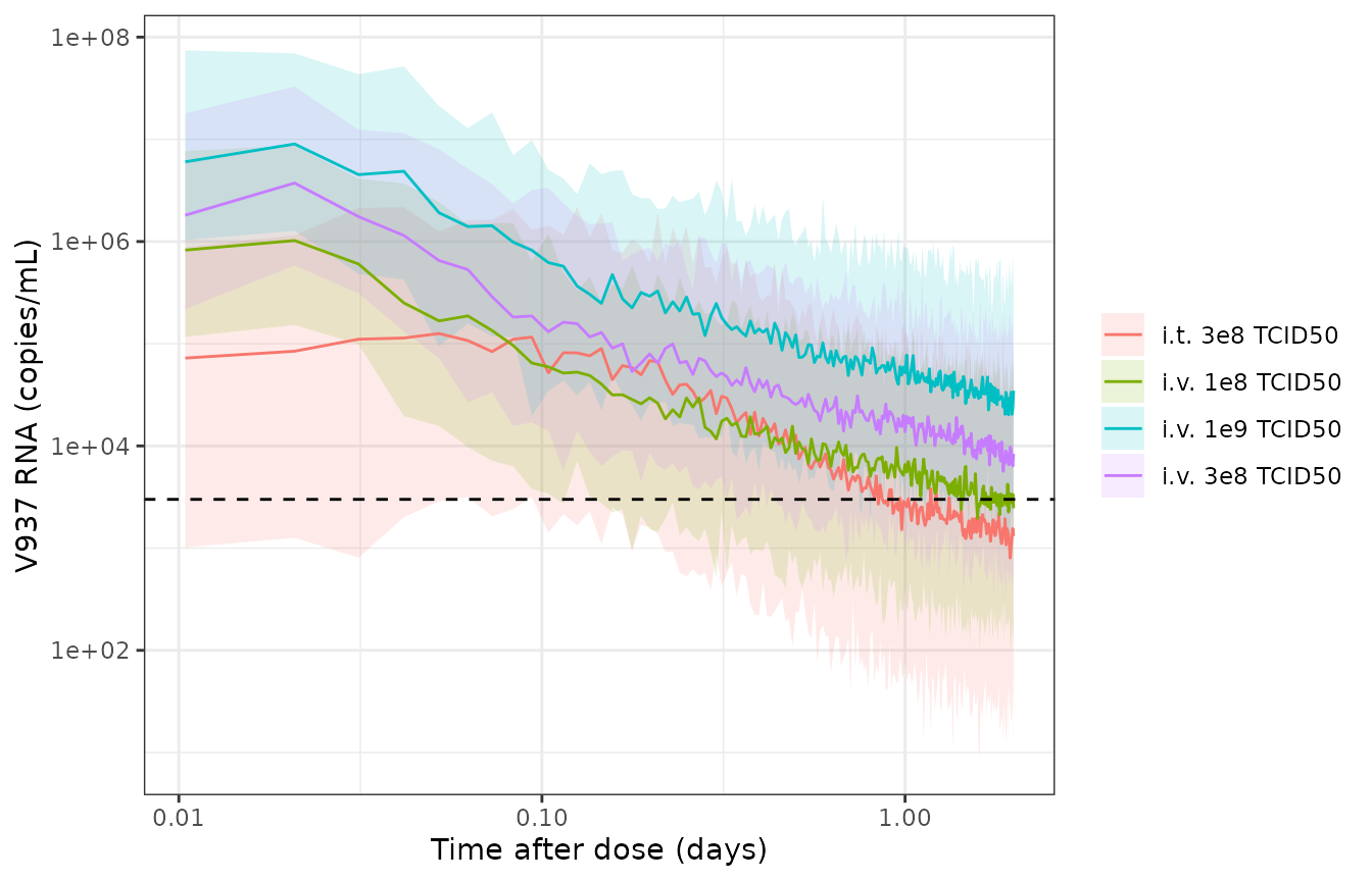
Serum V937 over the first 48 h (before the second dose): median and 5th-95th percentiles of simulated observations by arm; dashed line = 3000 copies/mL detection limit. Compare Figure 2A of Parra-Guillen 2025.
Figure 2A pools all arms and is prediction-corrected, so the comparison is visual. The observed data sit between about 10^4 and 10^7 copies/mL in the first hours after dosing, and the fraction below the detection limit climbs from near zero at about 0.1 day to roughly 45% at about 2 days and 100% beyond a week. The simulated pooled percentage below the limit follows the same course:
bld <- sim |>
  filter(time %in% c(2.5, 24, 47.75)) |>
  group_by(time) |>
  summarise(`% below 3000 copies/mL` = round(100 * mean(Cc_obs < 3000), 1), .groups = "drop") |>
  rename(`Time after first dose (h)` = time)
knitr::kable(bld)| Time after first dose (h) | % below 3000 copies/mL |
|---|---|
| 2.50 | 4.0 |
| 24.00 | 28.2 |
| 47.75 | 41.5 |
ADA over time (Fig. 2B)
ada_sum <- sim |>
  filter(time %% 24 == 0) |>
  group_by(arm, day) |>
  summarise(med = median(ada_obs), lo = quantile(ada_obs, 0.05), hi = quantile(ada_obs, 0.95),
            pct_bld = 100 * mean(ada_obs < 16), .groups = "drop")

ggplot(ada_sum, aes(day, med, colour = arm, fill = arm)) +
  geom_ribbon(aes(ymin = lo, ymax = hi), alpha = 0.12, colour = NA) +
  geom_line() +
  geom_hline(yintercept = 16, linetype = "dotted") +
  scale_y_log10() +
  labs(x = "Time after first dose (days)", y = "ADA (1/DL)", colour = NULL, fill = NULL) +
  theme_bw()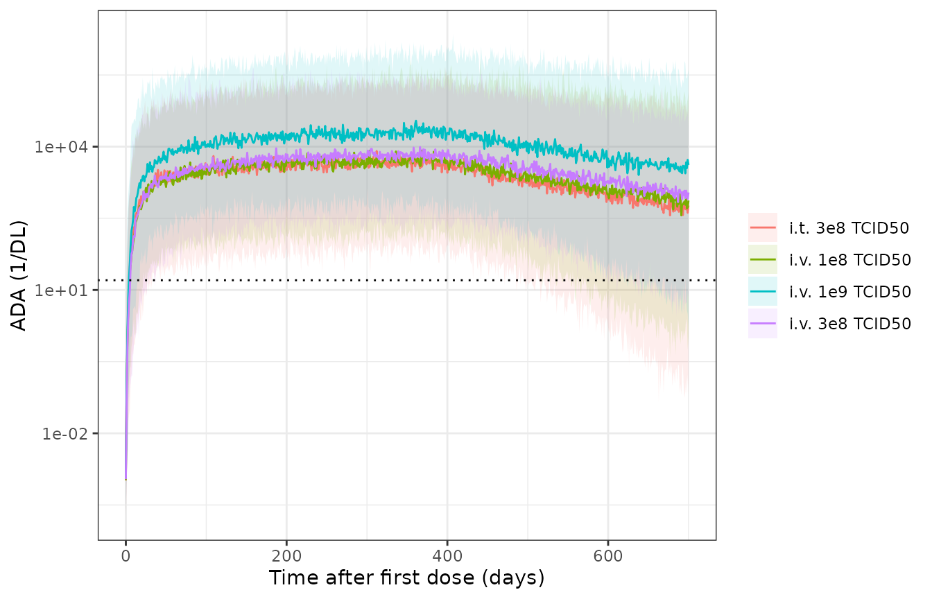
Neutralising ADA titre (dilution factor): median and 5th-95th percentiles of simulated observations by arm; dotted line = 1:16 detection limit. Compare Figure 2B of Parra-Guillen 2025.
In Figure 2B the observed median ADA rises within the first month to between roughly 10^3 and 10^4 and stays there, with fewer than about 10% of samples below the 1:16 limit after the first month. The simulated pooled cohort is checked against that plateau and that rise:
pooled <- sim |>
  filter(time %% 24 == 0, day %in% c(0, 7, 30, 100, 200, 300)) |>
  group_by(day) |>
  summarise(median_ada = signif(median(ada_obs), 3),
            pct_below_16 = round(100 * mean(ada_obs < 16), 1), .groups = "drop")
knitr::kable(pooled |> rename(`Day` = day, `Median ADA (DF)` = median_ada,
`% below 1:16` = pct_below_16))| Day | Median ADA (DF) | % below 1:16 |
|---|---|---|
| 0 | 1.06e-03 | 100.0 |
| 7 | 7.50e+01 | 31.5 |
| 30 | 1.82e+03 | 4.5 |
| 100 | 4.85e+03 | 1.2 |
| 200 | 6.23e+03 | 0.0 |
| 300 | 8.15e+03 | 0.5 |
plateau <- pooled |> filter(day %in% c(100, 200, 300))
stopifnot(
  # Before dosing every naive subject sits at the 0.001 offset.
  pooled$pct_below_16[pooled$day == 0] == 100,
  # Plateau median within the 10^3 - 10^4 band of Fig. 2B (a factor of 3
  # either side for the prediction correction and the arm mix).
  all(plateau$median_ada > 300),
  all(plateau$median_ada < 3e4),
  # Fewer than a fifth of samples below the limit once ADA is established.
  all(plateau$pct_below_16 < 20)
)
Pre-existing ADA
The paper adds an individual’s observed baseline titre to the predicted ADA when it is at or above 1:16, and ignores values below that limit. With the same individual parameters the three scenarios therefore differ by exactly the offset:
base_ev <- bind_rows(lapply(c(0, 8, 64), function(b) {
  make_arm(paste("ADA_TITER_BASE =", b), "i.v.", 3e8, 1, 0L) |>
    mutate(ADA_TITER_BASE = b, id = match(b, c(0, 8, 64)))
}))
# The three subjects share the typical parameters on purpose, so rxode2's
# "multi-subject simulation without 'omega'" warning is expected; only that
# warning is muffled.
base_sim <- withCallingHandlers(
  rxode2::rxSolve(rxode2::zeroRe(mod), base_ev, keep = "ADA_TITER_BASE",
                  returnType = "data.frame", useLinCmt = FALSE),
  warning = function(w) {
    if (grepl("without 'omega'", conditionMessage(w), fixed = TRUE)) invokeRestart("muffleWarning")
  }
) |>
  filter(!duplicated(paste(id, time)))
#> ℹ omega/sigma items treated as zero: 'etalcl', 'etalogitfdepot', 'etalksyn', 'etalktr', 'etalkdeg'
offset <- base_sim |>
  group_by(time) |>
  summarise(d8 = ada_total[ADA_TITER_BASE == 8] - ada_total[ADA_TITER_BASE == 0],
            d64 = ada_total[ADA_TITER_BASE == 64] - ada_total[ADA_TITER_BASE == 0],
            .groups = "drop")
stopifnot(max(abs(offset$d8)) < 1e-6, max(abs(offset$d64 - 64)) < 1e-6)
knitr::kable(data.frame(Scenario = c("ADA_TITER_BASE = 8 (below 1:16)", "ADA_TITER_BASE = 64"),
                        `Added to predicted ADA` = c(max(abs(offset$d8)), mean(offset$d64)),
check.names = FALSE))| Scenario | Added to predicted ADA |
|---|---|
| ADA_TITER_BASE = 8 (below 1:16) | 0 |
| ADA_TITER_BASE = 64 | 64 |
PKNCA validation
The paper reports no NCA, so the check is internal: after a single
dose, AUC0-inf must equal F * Dose / CL for each subject
(F = 1 i.v., F = FIT i.t.). A single dose with
a 7-day window is simulated per arm.
sd_events <- bind_rows(lapply(seq_along(c("i.t.", "i.v.", "i.v.", "i.v.")), function(k) {
  route <- c("i.t.", "i.v.", "i.v.", "i.v.")[k]
  tcid <- c(3e8, 1e8, 3e8, 1e9)[k]
  ids <- (k - 1L) * 100L + seq_len(100)
  obs_h <- sort(unique(c(0, 0.25, 0.5, 0.75, 1, 1.5, 2, 3, 4, 6, 8, 12, 16, 24, 36, 48, 72, 96, 120, 144, 168)))
  bind_rows(
    data.frame(id = ids, time = 0, evid = 1L, amt = tcid * copies_per_tcid50,
               cmt = if (route == "i.t.") "peripheral1" else "central",
               dur = if (route == "i.t.") 0 else 0.5, dvid = NA_integer_),
    expand.grid(id = ids, time = obs_h) |>
      mutate(evid = 0L, amt = 0, cmt = "central", dur = 0, dvid = 1L)
  ) |>
    mutate(treatment = paste(route, format(tcid, scientific = TRUE), "TCID50"), ADA_TITER_BASE = 0)
})) |> arrange(id, time, desc(evid))

sd_sim <- rxode2::rxSolve(mod, sd_events, keep = "treatment", returnType = "data.frame",
                          useLinCmt = FALSE) |>
  filter(!duplicated(paste(id, time)))

sim_nca <- sd_sim |>
  filter(!is.na(Cc)) |>
  select(id, time, Cc, treatment)
sim_nca <- bind_rows(sim_nca, sim_nca |> distinct(id, treatment) |> mutate(time = 0, Cc = 0)) |>
  distinct(id, treatment, time, .keep_all = TRUE) |>
  arrange(id, treatment, time)

conc_obj <- PKNCA::PKNCAconc(sim_nca, Cc ~ time | treatment + id)
dose_df <- sd_events |>
  filter(evid == 1) |>
  select(id, time, amt, treatment)
dose_obj <- PKNCA::PKNCAdose(dose_df, amt ~ time | treatment + id)
intervals <- data.frame(start = 0, end = Inf, cmax = TRUE, tmax = TRUE,
                        aucinf.obs = TRUE, half.life = TRUE)
nca_res <- PKNCA::pk.nca(PKNCA::PKNCAdata(conc_obj, dose_obj, intervals = intervals))

nca_tab <- as.data.frame(nca_res$result) |>
  filter(PPTESTCD %in% c("cmax", "tmax", "aucinf.obs", "half.life")) |>
  group_by(treatment, PPTESTCD) |>
  summarise(median = signif(median(PPORRES, na.rm = TRUE), 3), .groups = "drop") |>
  tidyr::pivot_wider(names_from = PPTESTCD, values_from = median)
knitr::kable(nca_tab |> rename(`Treatment` = treatment, `Cmax (copies/mL)` = cmax,
                               `Tmax (h)` = tmax, `AUC0-inf (copies*h/mL)` = aucinf.obs,
                               `t1/2 (h)` = half.life),
caption = "Median single-dose NCA of the simulated cohort (no published NCA to compare).")| Treatment | AUC0-inf (copies*h/mL) | Cmax (copies/mL) | t1/2 (h) | Tmax (h) |
|---|---|---|---|---|
| i.t. 3e+08 TCID50 | 706000 | 110000 | 23.1 | 1.0 |
| i.v. 1e+08 TCID50 | 1310000 | 1060000 | 23.2 | 0.5 |
| i.v. 1e+09 TCID50 | 13400000 | 10700000 | 23.3 | 0.5 |
| i.v. 3e+08 TCID50 | 3890000 | 3180000 | 23.1 | 0.5 |
# Closed-form AUC per subject: F * Dose / CL, converted from copies*h/L to
# copies*h/mL.
indiv <- sd_sim |>
  group_by(id) |>
  summarise(cl = first(cl), fit = first(fit), .groups = "drop")
auc_chk <- as.data.frame(nca_res$result) |>
  filter(PPTESTCD == "aucinf.obs") |>
  left_join(indiv, by = "id") |>
  left_join(dose_df |> select(id, amt), by = "id") |>
  mutate(f = ifelse(grepl("^i.t.", treatment), fit, 1),
         auc_ref = f * amt / cl / 1000,
         pct_diff = 100 * (PPORRES - auc_ref) / auc_ref)
knitr::kable(auc_chk |> group_by(treatment) |>
               summarise(`Median % difference, PKNCA vs F*Dose/CL` = round(median(pct_diff), 2),
                         .groups = "drop") |>
rename(`Treatment` = treatment))| Treatment | Median % difference, PKNCA vs F*Dose/CL |
|---|---|
| i.t. 3e+08 TCID50 | 0.21 |
| i.v. 1e+08 TCID50 | -0.08 |
| i.v. 1e+09 TCID50 | -0.05 |
| i.v. 3e+08 TCID50 | -0.10 |
Assumptions and deviations
- TCID50-to-copies factor. The paper does not state the factor used to convert TCID50 doses into the RNA-copy dose units of the model. Simulations here use 1500 copies per TCID50, the virions-per-TCID50 ratio in the authors’ tumour-response code (ESM 4). Users with the factor from the original dataset should substitute it; the model itself takes doses in copies.
-
EC50 units. Table 2 gives EC50 = 0.754 x 10^8
copies/L, and ESM 2 applies it to
A(1)/V1(copies/L). The Results text quotes “7.54 x 10^7 copies/mL”; the table and code agree, so the model uses copies/L (7.54 x 10^4 copies/mL). -
IIV of FIT. Table 2 lists 4.17 for the IIV of the
logit-transformed FIT with a footnote describing a CV% formula. ESM 2,
which fixes every other PK value at its Table 2 estimate, sets
$OMEGA 4.17 FIXfor this term, so 4.17 is used as the logit-scale variance. The other IIV terms are CV% values converted withomega^2 = log(1 + CV^2), the inverse of the paper’sCV = sqrt(exp(omega^2) - 1); this reproduces the ESM 2 CL value (0.375) exactly. - Zero-concentration guard. ESM 2 sets serum concentrations below 10^-6 copies/L to zero before computing the B-cell drive. This is a numerical guard with no effect on the drive (it is 10^14 times below EC50) and is not reproduced.
-
0.001 offset. The ESM 2 predictions carry
+ 0.001inside the log for both endpoints, soCcandada_totalinclude it. It is 6 orders of magnitude below the V937 detection limit and 4 below the ADA detection limit. - Censoring. Observations below the detection limits were handled by the M3 likelihood during estimation. That is part of fitting, not of the model, and is not encoded.
- Pre-existing ADA. The paper reports that 20 patients (about 10%) had ADA above 1:16 at baseline but not the distribution of their titres, so the simulated cohort is ADA-naive; the offset behaviour is shown separately.
- Covariates. Route, combination with pembrolizumab and pre-existing ADA were screened on KSYN, KTR and KDEG (ESM 3) and none was retained.
- Tumour-response layer. The in-silico neutralisation exercise (Fig. 3, ESM 4) couples this ADA model to the Parra-Guillen 2023 physiologically based V937 framework, whose viral-dynamic, tumour and immune parameters are not printed in this paper. It is not included here.