Fluticasone furoate, umeclidinium and vilanterol in COPD (Mehta 2020)
Source:vignettes/articles/Mehta_2020_fluticasoneFuroate_umeclidinium_vilanterol.Rmd
Mehta_2020_fluticasoneFuroate_umeclidinium_vilanterol.RmdModel and source
- Citation: Mehta R, Farrell C, Hayes S, Birk R, Okour M, Lipson DA. Population Pharmacokinetic Analysis of Fluticasone Furoate/Umeclidinium Bromide/Vilanterol in Patients with Chronic Obstructive Pulmonary Disease. Clin Pharmacokinet. 2020;59(1):67-79. doi:10.1007/s40262-019-00794-w
- Article (open access): https://doi.org/10.1007/s40262-019-00794-w (PMC6995987)
Fluticasone furoate (FF, an inhaled corticosteroid), umeclidinium (UMEC, a long-acting muscarinic antagonist) and vilanterol (VI, a long-acting beta2-agonist) are given once daily as a fixed-dose triple combination from a single dry-powder inhaler (FF/UMEC/VI 100/62.5/25 ug). Mehta 2020 pools sparse and serial plasma concentrations from three Phase III COPD trials – FULFIL, IMPACT and study 200812 – that compared the single-inhaler triple against multiple-inhaler triple therapy (FF/VI + UMEC) and the dual combinations FF/VI and UMEC/VI. Each analyte was fitted separately in NONMEM (SAEM, M3 method for the 41% / 13% / 21% of FF / UMEC / VI records below the 10 pg/mL LLOQ).
The paper contains three independent models, one per analyte, each with its own dataset (Table 2) and parameter table (Tables 3, 6 and 9). They share no parameters, so they are extracted as three model files:
ff <- rxode2::rxode(readModelDb("Mehta_2020_fluticasoneFuroate"))
#> ℹ parameter labels from comments will be replaced by 'label()'
umec <- rxode2::rxode(readModelDb("Mehta_2020_umeclidinium"))
#> ℹ parameter labels from comments will be replaced by 'label()'
vi <- rxode2::rxode(readModelDb("Mehta_2020_vilanterol"))
#> ℹ parameter labels from comments will be replaced by 'label()'| Fluticasone furoate | Umeclidinium | Vilanterol | |
|---|---|---|---|
| Structure | 2-compartment, first-order absorption | 2-compartment, first-order absorption | 2-compartment, first-order absorption |
| Fixed THETAs | V2/F, Q/F, V3/F | Q/F, V3/F | KA |
| Covariates | Japanese heritage, FF/VI arm on CL/F | WT, age, smoking on CL/F; WT on V2/F | WT on CL/F; smoking on V2/F |
| Dataset | 714 subjects, 2948 obs, 41% BQL | 622 subjects, 2589 obs, 13% BQL | 817 subjects, 3331 obs, 21% BQL |
Units
All three files declare dosing = "ug" and volumes in L,
so Cc is in ug/L, i.e. ng/mL. Mehta 2020
reports every concentration and exposure in pg/mL and pg*h/mL, so the
vignette multiplies Cc by 1000 before any comparison. This
is the same convention as the Siederer 2016 FF and VI models of the same
lineage.
Population
714 (FF), 622 (UMEC) and 817 (VI) adults with symptomatic COPD at risk of exacerbation contributed PK data (Table 2). The three datasets overlap heavily: median age 66 years (41-88), median weight about 72 kg (35.4-154), 27-29% female, roughly two thirds White, 14-18% East Asian and 13-14% Japanese (all East Asian and Japanese subjects were resident in China, Japan or Korea), and 39-40% current smokers. Median percent-predicted FEV1 was 39.7%.
Source trace
| Quantity | Model file / parameter | Value | Source |
|---|---|---|---|
| FF CL/F | lcl |
513 L/h | Table 3; Sect. 3.2 |
| FF V2/F | lvc |
1.36 L (fixed) | Table 3; Sect. 3.2 |
| FF Q/F | lq |
268 L/h (fixed) | Table 3 |
| FF V3/F | lvp |
111 L (fixed) | Table 3 |
| FF KA | lka |
0.0821 1/h | Table 3 |
| FF Japanese heritage on CL/F | e_race_japanese_cl |
-0.436 (x0.647) | Table 3; Sect. 3.2 ‘35% lower’ |
| FF FF/VI arm on CL/F | e_ffvi_cl |
0.351 (x1.42) | Table 3; Sect. 3.2 ‘42% higher’ |
| FF IIV CL, V2, Q, V3, KA |
etalcl … etalka
|
69.2, 397, 77.3, 67.8, 70.6 CV% | Table 3 |
| UMEC CL/F | lcl |
149 L/h | Table 6; Sect. 3.2 |
| UMEC V2/F | lvc |
1100 L | Table 6 |
| UMEC Q/F | lq |
854 L/h (fixed) | Table 6 |
| UMEC V3/F | lvp |
16,200 L (fixed) | Table 6 |
| UMEC KA | lka |
18.6 1/h | Table 6 |
| UMEC WT on CL/F | e_wt_cl |
0.580 | Table 6 |
| UMEC age on CL/F | e_age_cl |
-0.648 | Table 6 |
| UMEC smoking on CL/F | e_smoke_cl |
log(1.28) | Table 6 |
| UMEC WT on V2/F | e_wt_vc |
0.797 | Table 6 |
| UMEC IIV CL, V2, Q, V3, KA |
etalcl … etalka
|
37.7, 51.5, 66.9, 80.4, 65.0 CV% | Table 6 |
| VI CL/F | lcl |
73.5 L/h | Table 9; Sect. 3.3 |
| VI V2/F | lvc |
352 L | Table 9; Sect. 3.3 |
| VI Q/F | lq |
242 L/h | Table 9 |
| VI V3/F | lvp |
2250 L | Table 9 |
| VI KA | lka |
19.6 1/h (fixed) | Table 9; Sect. 3.3 |
| VI WT on CL/F | e_wt_cl |
0.444 | Table 9 |
| VI smoking on V2/F | e_smoke_vc |
log(1.46) | Table 9 |
| VI IIV CL, V2, Q, V3, KA |
etalcl … etalka
|
28.8, 44.5, 17.2, 98.7, 41.4 CV% | Table 9 |
| Continuous covariate form |
(COV/REF)^theta, REF 70 kg / 60 y |
– | Eq. 1; Sect. 3.2-3.3 typical-value statements |
| Categorical covariate form | theta^CAT |
– | Eq. 2 |
| Structure (all three) | 2-cmt, first-order absorption and elimination | – | Sect. 3.2, 3.3 |
| Residual error (all three) |
propSd fixed(0) |
not reported | see Assumptions |
Covariate effects: the paper’s own quoted percentages
Sect. 3.2 and 3.3 translate every covariate estimate into a
percentage change for a named subject. These are deterministic functions
of the ini() values and pin both the functional form (power
vs linear) and the reference values (70 kg, 60 years).
p_ff <- ff$theta
p_um <- umec$theta
p_vi <- vi$theta
claims <- tibble::tribble(
  ~Claim, ~Paper_pct, ~Model_pct,
  "FF CL/F, Japanese heritage (35% lower)", -35, 100 * (exp(p_ff[["e_race_japanese_cl"]]) - 1),
  "FF CL/F, FF/VI arm (42% higher)", 42, 100 * (exp(p_ff[["e_ffvi_cl"]]) - 1),
  "UMEC CL/F, smoker (28% higher)", 28, 100 * (exp(p_um[["e_smoke_cl"]]) - 1),
  "UMEC CL/F, 80 vs 60 years (17% lower)", -17, 100 * ((80 / 60)^p_um[["e_age_cl"]] - 1),
  "UMEC CL/F, +10% age (about 6% lower)", -6, 100 * (1.1^p_um[["e_age_cl"]] - 1),
  "UMEC CL/F, +10% weight (about 6% higher)", 6, 100 * (1.1^p_um[["e_wt_cl"]] - 1),
  "UMEC V2/F, +10% weight (8% higher)", 8, 100 * (1.1^p_um[["e_wt_vc"]] - 1),
  "UMEC CL/F, 100 vs 70 kg (23% higher)", 23, 100 * ((100 / 70)^p_um[["e_wt_cl"]] - 1),
  "UMEC V2/F, 100 vs 70 kg (33% higher)", 33, 100 * ((100 / 70)^p_um[["e_wt_vc"]] - 1),
  "UMEC V2/F, 40 vs 70 kg (36% lower)", -36, 100 * ((40 / 70)^p_um[["e_wt_vc"]] - 1),
  "UMEC CL/F, 40 vs 70 kg (32% lower)", -32, 100 * ((40 / 70)^p_um[["e_wt_cl"]] - 1),
  "VI CL/F, +10% weight (about 4% higher)", 4, 100 * (1.1^p_vi[["e_wt_cl"]] - 1),
  "VI CL/F, 40 vs 70 kg (22% lower)", -22, 100 * ((40 / 70)^p_vi[["e_wt_cl"]] - 1),
  "VI CL/F, 100 vs 70 kg (17% higher)", 17, 100 * ((100 / 70)^p_vi[["e_wt_cl"]] - 1),
  "VI V2/F, smoker (46% higher)", 46, 100 * (exp(p_vi[["e_smoke_vc"]]) - 1)
) |>
  mutate(
    Model_pct = round(Model_pct, 1),
    Diff = Model_pct - Paper_pct,
    # The one known disagreement: see below.
    Deviation = grepl("CL/F, 40 vs 70 kg \\(32%", Claim)
  )
claims |>
  dplyr::rename(
    "Paper (%)" = Paper_pct, "Model (%)" = Model_pct,
    "Model - paper (points)" = Diff, "Known deviation" = Deviation
  ) |>
knitr::kable()| Claim | Paper (%) | Model (%) | Model - paper (points) | Known deviation |
|---|---|---|---|---|
| FF CL/F, Japanese heritage (35% lower) | -35 | -35.3 | -0.3 | FALSE |
| FF CL/F, FF/VI arm (42% higher) | 42 | 42.0 | 0.0 | FALSE |
| UMEC CL/F, smoker (28% higher) | 28 | 28.0 | 0.0 | FALSE |
| UMEC CL/F, 80 vs 60 years (17% lower) | -17 | -17.0 | 0.0 | FALSE |
| UMEC CL/F, +10% age (about 6% lower) | -6 | -6.0 | 0.0 | FALSE |
| UMEC CL/F, +10% weight (about 6% higher) | 6 | 5.7 | -0.3 | FALSE |
| UMEC V2/F, +10% weight (8% higher) | 8 | 7.9 | -0.1 | FALSE |
| UMEC CL/F, 100 vs 70 kg (23% higher) | 23 | 23.0 | 0.0 | FALSE |
| UMEC V2/F, 100 vs 70 kg (33% higher) | 33 | 32.9 | -0.1 | FALSE |
| UMEC V2/F, 40 vs 70 kg (36% lower) | -36 | -36.0 | 0.0 | FALSE |
| UMEC CL/F, 40 vs 70 kg (32% lower) | -32 | -27.7 | 4.3 | TRUE |
| VI CL/F, +10% weight (about 4% higher) | 4 | 4.3 | 0.3 | FALSE |
| VI CL/F, 40 vs 70 kg (22% lower) | -22 | -22.0 | 0.0 | FALSE |
| VI CL/F, 100 vs 70 kg (17% higher) | 17 | 17.2 | 0.2 | FALSE |
| VI V2/F, smoker (46% higher) | 46 | 46.0 | 0.0 | FALSE |
# Deterministic: every value is a closed-form function of the ini() values,
# so a tight bound is correct. The paper rounds to whole percent.
stopifnot(all(abs(claims$Diff[!claims$Deviation]) < 1))
Fourteen of the fifteen quoted percentages reproduce to within
rounding. The exception is “A 40-kg subject with COPD would have a 32%
lower CL/F” for UMEC: (40/70)^0.580 gives a 27.7%
reduction. The same sentence’s companion values (36% lower V2/F at 40
kg, 23% / 33% higher CL/F / V2/F at 100 kg) all reproduce with the 70 kg
reference and the Table 6 exponents, and no single reference weight or
exponent reproduces 32% together with the others, so this is treated as
a misprint in the prose rather than a parameter error.
Typical-value steady-state exposure
Sect. 2.6 defines AUC(0-24) = dose / (CL/F) and simulates steady-state Cmax. For the reference subject of each model (FF: non-Japanese, UMEC co-administered; UMEC: 60 years, 70 kg, non-smoker; VI: 70 kg, non-smoker) the typical profile over the 90th daily dose is (90 days, because the UMEC peripheral volume of 16,200 L – larger still with IIV – gives a terminal half-life of days):
doses <- c(FF = 100, UMEC = 62.5, VI = 25)
ref_cov <- data.frame(WT = 70, AGE = 60, SMOKE = 0, RACE_JAPANESE = 0, CONMED_UMECLIDINIUM = 1)
obs_tad <- c(0, 0.05, 0.1, 0.15, 0.2, 0.25, 0.33, 0.5, 0.75, 1, 1.25, 1.5, 2, 2.5, 3, 4, 5, 6, 8, 10, 12, 16, 20, 24)
t_last <- 89 * 24
ev_typ <- function(dose) {
  et(amt = dose, cmt = "depot", ii = 24, addl = 89) |>
    et(t_last + obs_tad, cmt = "central")
}
typ <- bind_rows(
  as.data.frame(rxSolve(rxode2::zeroRe(ff), ev_typ(doses[["FF"]]), params = ref_cov)) |> mutate(drug = "FF"),
  as.data.frame(rxSolve(rxode2::zeroRe(umec), ev_typ(doses[["UMEC"]]), params = ref_cov)) |> mutate(drug = "UMEC"),
  as.data.frame(rxSolve(rxode2::zeroRe(vi), ev_typ(doses[["VI"]]), params = ref_cov)) |> mutate(drug = "VI")
) |>
  mutate(tad = time - t_last, Cc_pg = 1000 * Cc)
#> ℹ omega/sigma items treated as zero: 'etalcl', 'etalvc', 'etalq', 'etalvp', 'etalka'
#> ℹ omega/sigma items treated as zero: 'etalcl', 'etalvc', 'etalq', 'etalvp', 'etalka'
#> ℹ omega/sigma items treated as zero: 'etalcl', 'etalvc', 'etalq', 'etalvp', 'etalka'

typ_sum <- typ |>
  group_by(drug) |>
  summarise(
    cmax = max(Cc_pg),
    auc = sum(diff(tad) * (head(Cc_pg, -1) + tail(Cc_pg, -1)) / 2),
    .groups = "drop"
  ) |>
  mutate(
    auc_closed = 1000 * doses[drug] / exp(c(ff$theta[["lcl"]], umec$theta[["lcl"]], vi$theta[["lcl"]])),
    # Published geometric means for the subgroup closest to the reference
    # subject: FF White FF/UMEC/VI (Table 4); UMEC former smoker FF/UMEC/VI
    # (Table 7); VI former smoker FF/UMEC/VI (Table 10).
    cmax_paper = c(17.6, 63.2, 77.5),
    auc_paper = c(215, 457, 369)
  )
typ_sum |>
  mutate(across(where(is.numeric), \(x) signif(x, 3))) |>
  dplyr::rename(
    "Analyte" = drug, "Cmax,ss (pg/mL)" = cmax, "AUC0-24 trapezoid (pg*h/mL)" = auc,
    "AUC0-24 = dose/CL (pg*h/mL)" = auc_closed, "Paper Cmax" = cmax_paper, "Paper AUC0-24" = auc_paper
  ) |>
knitr::kable()| Analyte | Cmax,ss (pg/mL) | AUC0-24 trapezoid (pg*h/mL) | AUC0-24 = dose/CL (pg*h/mL) | Paper Cmax | Paper AUC0-24 |
|---|---|---|---|---|---|
| FF | 16.3 | 195 | 195 | 17.6 | 215 |
| UMEC | 62.3 | 420 | 419 | 63.2 | 457 |
| VI | 69.7 | 341 | 340 | 77.5 | 369 |
# Numerical vs closed form on the same parameters: pure solver/trapezoid error.
stopifnot(all(abs(typ_sum$auc / typ_sum$auc_closed - 1) < 0.01))
The typical AUCs equal dose/CL by construction (a check on the
steady-state solve). They sit 8-10% below the published subgroup
geometric means for all three analytes because the published values are
geometric means of post-hoc individual estimates across subjects who
differ from the reference (median age 66 years, not 60, for UMEC:
(66/60)^-0.648 alone raises AUC 6%).
ggplot(typ, aes(tad, Cc_pg)) +
  geom_line() +
  geom_hline(yintercept = 10, linetype = "dashed", colour = "red") +
  facet_wrap(~drug, scales = "free_y") +
  labs(x = "Time after dose (h)", y = "Concentration (pg/mL)")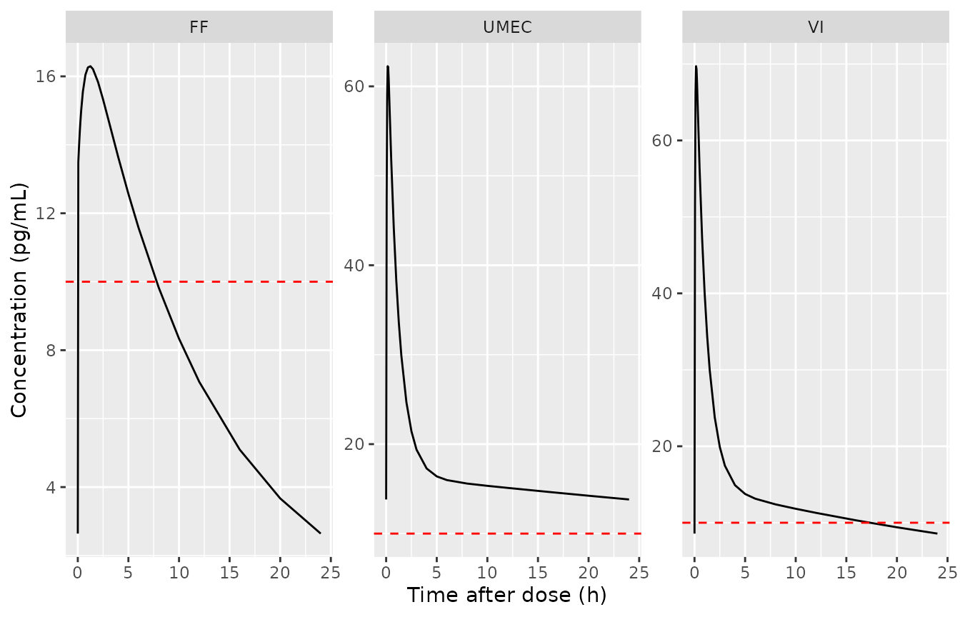
Typical steady-state profiles over one dosing interval (reference subject of each model). Dashed line: 10 pg/mL LLOQ. Compare the medians of Figs. 3, 6 and 9 of Mehta 2020.
Virtual cohort and VPC-style simulation
A cohort resembling Table 2 is drawn for each analyte: body weight log-normal around the 72 kg median, truncated to the observed 35.4-154 kg; age normal around the 66-year median (SD 8), truncated to 41-88 years; 40% current smokers; 13% Japanese heritage. The FF cohort has two arms of 200 – FF/UMEC/VI (and FF/VI + UMEC, which share the reference) and FF/VI – because the arm is an FF covariate. UMEC and VI have no treatment covariate, so each has one cohort of 200, summarised by smoking status for comparison with Tables 7 and 10.
rxode2::rxSetSeed(20200719)
make_cohort <- function(n, arm, id0 = 0) {
  data.frame(
    id = id0 + seq_len(n),
    arm = arm,
    WT = pmin(pmax(exp(rnorm(n, log(72), 0.2)), 35.4), 154),
    AGE = pmin(pmax(rnorm(n, 66, 8), 41), 88),
    SMOKE = rbinom(n, 1, 0.40),
    RACE_JAPANESE = rbinom(n, 1, 0.13),
    CONMED_UMECLIDINIUM = as.integer(arm != "FF/VI")
  )
}
set.seed(20200719)
cohort_ff <- bind_rows(make_cohort(200, "FF/UMEC/VI"), make_cohort(200, "FF/VI", id0 = 200))
cohort_um <- make_cohort(200, "FF/UMEC/VI")
cohort_vi <- make_cohort(200, "FF/UMEC/VI")

make_events <- function(cohort, dose) {
  dose_rows <- cohort |>
    tidyr::crossing(time = seq(0, t_last, by = 24)) |>
    mutate(evid = 1, amt = dose, cmt = "depot")
  obs_rows <- cohort |>
    tidyr::crossing(time = t_last + obs_tad) |>
    mutate(evid = 0, amt = 0, cmt = "central")
  bind_rows(dose_rows, obs_rows) |>
    arrange(id, time, desc(evid)) |>
    select(-arm)
}

sim_cohort <- function(mod, cohort, dose, drug) {
  s <- rxSolve(mod, make_events(cohort, dose), returnType = "data.frame")
  # rxSolve returns the covariates each model uses; drop them so the cohort's
  # own columns (the same for every analyte) join back without .x / .y pairs.
  s |>
    select(-any_of(c("WT", "AGE", "SMOKE", "RACE_JAPANESE", "CONMED_UMECLIDINIUM"))) |>
    left_join(cohort |> select(id, arm, SMOKE, RACE_JAPANESE), by = "id") |>
    mutate(tad = time - t_last, Cc_pg = 1000 * Cc, drug = drug)
}
sims <- bind_rows(
  sim_cohort(ff, cohort_ff, doses[["FF"]], "FF"),
  sim_cohort(umec, cohort_um, doses[["UMEC"]], "UMEC"),
  sim_cohort(vi, cohort_vi, doses[["VI"]], "VI")
)
vpc <- sims |>
  group_by(drug, tad) |>
  summarise(
    p05 = quantile(Cc_pg, 0.05), p50 = median(Cc_pg), p95 = quantile(Cc_pg, 0.95),
    .groups = "drop"
  )
ggplot(vpc, aes(tad)) +
  geom_ribbon(aes(ymin = p05, ymax = p95), fill = "steelblue", alpha = 0.3) +
  geom_line(aes(y = p50), colour = "blue") +
  geom_hline(yintercept = 10, linetype = "dashed", colour = "red") +
  facet_wrap(~drug, scales = "free_y") +
  labs(x = "Time after dose (h)", y = "Concentration (pg/mL)")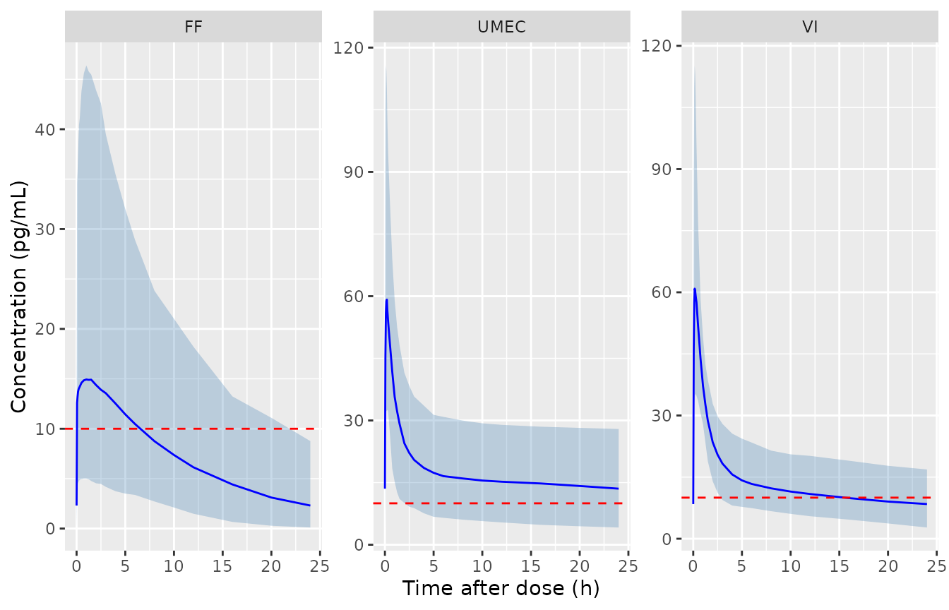
Simulated steady-state 5th, 50th and 95th percentiles (shaded 90% interval) over one dosing interval. Replicates the layout of Figs. 3 (FF), 6 (UMEC) and 9 (VI) of Mehta 2020; the red dashed line is the 10 pg/mL LLOQ.
Proportion below the LLOQ
Table 5 compares observed and predicted percentages of BQL data by time window. The simulated percentages below use the same windows.
bql <- sims |>
  filter(tad > 0) |>
  mutate(window = cut(tad, c(0, 0.5, 2, 5, 9, 20, 24), labels = c("0-0.5", "0.5-2", "2-5", "5-9", "9-20", ">20"), include.lowest = TRUE)) |>
  group_by(drug, window) |>
  summarise(sim_pct = round(100 * mean(Cc_pg < 10)), .groups = "drop") |>
  left_join(
    tibble::tibble(
      drug = rep(c("FF", "UMEC", "VI"), each = 6),
      window = rep(c("0-0.5", "0.5-2", "2-5", "5-9", "9-20", ">20"), 3),
      obs_pct = c(33, 16, 19, 43, 59, 79, 4, 5, 16, 29, 30, 33, 6, 5, 5, 22, 39, 62),
      paper_pred_pct = c(33, 24, 28, 43, 56, 78, 3, 5, 16, 29, 34, 40, 5, 6, 23, 40, 47, 62)
    ),
    by = c("drug", "window")
  )
bql |>
  dplyr::rename(
    "Analyte" = drug, "Window (h)" = window, "Simulated here (%)" = sim_pct,
    "Observed, Table 5 (%)" = obs_pct, "Predicted, Table 5 (%)" = paper_pred_pct
  ) |>
knitr::kable()| Analyte | Window (h) | Simulated here (%) | Observed, Table 5 (%) | Predicted, Table 5 (%) |
|---|---|---|---|---|
| FF | 0-0.5 | 27 | 33 | 33 |
| FF | 0.5-2 | 26 | 16 | 24 |
| FF | 2-5 | 35 | 19 | 28 |
| FF | 5-9 | 54 | 43 | 43 |
| FF | 9-20 | 83 | 59 | 56 |
| FF | >20 | 96 | 79 | 78 |
| UMEC | 0-0.5 | 0 | 4 | 3 |
| UMEC | 0.5-2 | 2 | 5 | 5 |
| UMEC | 2-5 | 11 | 16 | 16 |
| UMEC | 5-9 | 20 | 29 | 29 |
| UMEC | 9-20 | 27 | 30 | 34 |
| UMEC | >20 | 34 | 33 | 40 |
| VI | 0-0.5 | 0 | 6 | 5 |
| VI | 0.5-2 | 0 | 5 | 6 |
| VI | 2-5 | 8 | 5 | 23 |
| VI | 5-9 | 23 | 22 | 40 |
| VI | 9-20 | 46 | 39 | 47 |
| VI | >20 | 66 | 62 | 62 |
The simulated BQL fractions follow the published model-predicted fractions in shape (FF is the most censored analyte and its trough is mostly BQL; UMEC the least). They are not expected to match exactly: the paper’s predictions include residual error, the real sampling times and the real covariate distribution, none of which is reproduced here (the residual error is not reported; see Assumptions). The largest gap is FF after 9 h, where the simulated individual predictions are BQL more often than the paper’s predictions: FF typical concentrations sit only just above 10 pg/mL late in the interval (figure above), so residual error – absent here – scatters a material share of simulated observations back above the LLOQ.
PKNCA validation
conc_df <- sims |>
  filter(!is.na(Cc)) |>
  mutate(group = paste(drug, arm, ifelse(SMOKE == 1, "Current", "Former"), sep = " | ")) |>
  select(id, drug, arm, SMOKE, group, tad, Cc_pg)
dose_df <- conc_df |>
  distinct(id, drug, arm, SMOKE, group) |>
  mutate(tad = 0, amt = doses[drug])

conc_obj <- PKNCAconc(conc_df, Cc_pg ~ tad | drug + arm + id)
dose_obj <- PKNCAdose(dose_df, amt ~ tad | drug + arm + id)
intervals <- data.frame(start = 0, end = 24, cmax = TRUE, auclast = TRUE)
nca <- pk.nca(PKNCAdata(conc_obj, dose_obj, intervals = intervals))
nca_ind <- as.data.frame(nca$result) |>
  select(id, drug, arm, PPTESTCD, PPORRES) |>
  left_join(conc_df |> distinct(id, drug, SMOKE), by = c("id", "drug"))
Comparison against the published model-predicted exposures
Tables 4, 7, 8, 10 and 11 report geometric means of
model-predicted steady-state Cmax and AUC(0-24).
ncaComparisonTable() pools per-subject rows by the median,
so the simulated side is aggregated to geometric means first and passed
pre-aggregated.
geo <- function(x) exp(mean(log(x)))
overall_sim <- nca_ind |>
  group_by(drug, arm, PPTESTCD) |>
  summarise(PPORRES = geo(PPORRES), .groups = "drop") |>
  mutate(group = paste(drug, arm, "overall"))
smoke_sim <- nca_ind |>
  filter(drug %in% c("UMEC", "VI")) |>
  group_by(drug, arm, SMOKE, PPTESTCD) |>
  summarise(PPORRES = geo(PPORRES), .groups = "drop") |>
  mutate(group = paste(drug, arm, ifelse(SMOKE == 1, "current smoker", "former smoker")))
sim_tab <- bind_rows(overall_sim, smoke_sim) |> select(group, PPTESTCD, PPORRES)

ref_tab <- tibble::tribble(
  ~group, ~cmax, ~auclast,
  "FF FF/UMEC/VI overall", 18.7, 230, # Table 4 Overall FF/UMEC/VI
  "FF FF/VI overall", 13.3, 158, # Table 4 Overall FF/VI
  "UMEC FF/UMEC/VI overall", 59.6, 405, # Table 8 Overall FF/UMEC/VI
  "UMEC FF/UMEC/VI former smoker", 63.2, 457, # Table 7
  "UMEC FF/UMEC/VI current smoker", 54.7, 341, # Table 7
  "VI FF/UMEC/VI overall", 67.4, 362, # Table 11 Overall FF/UMEC/VI
  "VI FF/UMEC/VI former smoker", 77.5, 369, # Table 10
  "VI FF/UMEC/VI current smoker", 55.1, 353 # Table 10
)
cmp <- ncaComparisonTable(
  simulated = sim_tab,
  reference = ref_tab,
  by = "group",
  tolerance_pct = 20,
  units = c(cmax = "pg/mL", auclast = "pg*h/mL")
)
knitr::kable(cmp)| NCA parameter | group | Reference | Simulated | % diff |
|---|---|---|---|---|
| Cmax (pg/mL) | FF FF/UMEC/VI overall | 18.7 | 17.1 | -8.8% |
| Cmax (pg/mL) | FF FF/VI overall | 13.3 | 14.3 | +7.6% |
| Cmax (pg/mL) | UMEC FF/UMEC/VI overall | 59.6 | 60.9 | +2.2% |
| Cmax (pg/mL) | UMEC FF/UMEC/VI former smoker | 63.2 | 64.9 | +2.6% |
| Cmax (pg/mL) | UMEC FF/UMEC/VI current smoker | 54.7 | 55.1 | +0.7% |
| Cmax (pg/mL) | VI FF/UMEC/VI overall | 67.4 | 63.2 | -6.2% |
| Cmax (pg/mL) | VI FF/UMEC/VI former smoker | 77.5 | 70.3 | -9.3% |
| Cmax (pg/mL) | VI FF/UMEC/VI current smoker | 55.1 | 54 | -2.0% |
| AUClast (pg*h/mL) | FF FF/UMEC/VI overall | 230 | 193 | -16.2% |
| AUClast (pg*h/mL) | FF FF/VI overall | 158 | 157 | -0.7% |
| AUClast (pg*h/mL) | UMEC FF/UMEC/VI overall | 405 | 395 | -2.5% |
| AUClast (pg*h/mL) | UMEC FF/UMEC/VI former smoker | 457 | 445 | -2.5% |
| AUClast (pg*h/mL) | UMEC FF/UMEC/VI current smoker | 341 | 326 | -4.4% |
| AUClast (pg*h/mL) | VI FF/UMEC/VI overall | 362 | 333 | -8.1% |
| AUClast (pg*h/mL) | VI FF/UMEC/VI former smoker | 369 | 329 | -11.0% |
| AUClast (pg*h/mL) | VI FF/UMEC/VI current smoker | 353 | 339 | -4.1% |
# "% diff" is formatted text such as "+7.6%" or "-21.3%*".
pct <- as.numeric(gsub("[%*+]", "", cmp[["% diff"]]))
stopifnot(!anyNA(pct), length(pct) == 2 * nrow(ref_tab))
# Structural gate on the centre of the comparison: a mis-transcribed
# clearance, dose or unit moves every row by tens of percent. The per-row
# spread reflects EBE shrinkage in the published post-hoc summaries and the
# approximated covariate distribution, not the parameters.
stopifnot(
  abs(median(pct)) < 15,
  quantile(abs(pct), 0.9) < 30
)
The directions the paper emphasises are reproduced: the FF/VI arm has lower FF exposure than the triple-therapy arm (for the same subject exactly 1/1.42, the Table 3 multiplier; the published overall geometric means give 230/158 = 1.46, and the ratio realised here also depends on each arm’s drawn Japanese fraction and CL/F etas); smoking lowers UMEC AUC (via CL/F) but leaves VI AUC nearly unchanged while lowering VI Cmax (via V2/F), as in Tables 7 and 10.
Assumptions and deviations
-
Residual error not reported. Mehta 2020 states the
estimation method (SAEM with interaction, M3 for BQL data) but never
names the residual-error model or reports its magnitude. Each model
declares
propSd <- fixed(0); simulations here are therefore of individual predictions. Users simulating observations must supply their own residual error. - IIV scale. Tables 3, 6 and 9 report IIV as CV%. These were converted to log-normal variances with omega^2 = log(1 + CV^2). The alternative reading (CV = 100 x omega) gives larger variances for the wide rows – most notably FF V2/F, 397 CV%, where it would give omega^2 = 15.8 instead of 2.82. No OMEGA estimates, RSEs of OMEGA, or control stream are published to discriminate the two; FF V2/F is a fixed, poorly informed central volume (1.36 L) whose IIV has little effect on the plasma profile.
- No IIV correlations are reported; all etas are independent.
-
FF treatment-arm covariate. The paper’s FF/VI
indicator is encoded as
1 - CONMED_UMECLIDINIUM(new canonical, registered ininst/references/covariate-columns.md), because both reference arms – single-inhaler FF/UMEC/VI and FF/VI + UMEC – contain umeclidinium. The indicator records arm assignment only; the paper proposes no mechanism. - Covariate references. Eq. 1 says REF is the dataset median, but the paper’s typical-value statements and every quoted percentage use 70 kg and 60 years; those are used here.
- UMEC 40 kg misprint. “A 40-kg subject … 32% lower CL/F” is inconsistent with the Table 6 exponent (27.7% reproduced) while every companion value in the same sentence reproduces; treated as a prose misprint (see above).
- Virtual cohort. Weight and age distributions are approximated from the Table 2 medians and ranges (the paper reports no SDs); the Japanese-heritage and smoker fractions are from Table 2.
- Doses are nominal: FF 100 ug, UMEC 62.5 ug (as umeclidinium), VI 25 ug once daily (Table 1).