Lamotrigine + N-2-glucuronide (Milosheska 2016)
Source:vignettes/articles/Milosheska_2016_lamotrigine.Rmd
Milosheska_2016_lamotrigine.RmdModel and source
#> ℹ parameter labels from comments will be replaced by 'label()'- Citation: Milosheska D, Lorber B, Vovk T, Kastelic M, Dolzan V, Grabnar I. Pharmacokinetics of lamotrigine and its metabolite N-2-glucuronide: Influence of polymorphism of UDP-glucuronosyltransferases and drug transporters. Br J Clin Pharmacol. 2016;82(2):399-411. doi:10.1111/bcp.12984.
- Description: One-compartment first-order-absorption parent + one-compartment metabolite population pharmacokinetic model for oral lamotrigine (LTG) and its N-2-glucuronide (LTG-glu) in 100 adult Slovenian epilepsy patients on stable mono- or adjunctive therapy (Milosheska 2016). Complete conversion of parent to metabolite is assumed (LTG-N-5-glucuronide is a minor route, < 10% urinary excretion of unchanged drug per the paper’s Discussion citing Ref [5]). Parent apparent oral clearance (CL/F) carries a power effect of total body weight and additive-in-fraction effects of smoking, concomitant enzyme-inducing antiepileptic drugs (carbamazepine, phenobarbital, or phenytoin, pooled as CONMED_EIAED), concomitant UGT2B7 inhibitors (valproic acid or sertraline, pooled as CONMED_UGT_INH), Cockcroft-Gault estimated creatinine clearance (deviation from 110 mL/min), and two UGT2B7 SNP genotype categoricals (-161C>T rs7668258 and 372A>G rs28365063). Parent apparent volume (V/F) carries a linear deviation-from-reference weight effect. Metabolite apparent clearance (CL_LTG-glu / F_metab) carries a power weight and linear Cockcroft-Gault CLcr effect; metabolite apparent volume (V_LTG-glu / F_metab) is estimated as a typical value only (no IIV supported by the sparse metabolite data).
- Article: https://doi.org/10.1111/bcp.12984
The packaged model implements the Milosheska 2016 parent + metabolite
joint population-PK model for oral lamotrigine (LTG) and its
N-2-glucuronide (LTG-glu) in adult epilepsy patients. The parent side is
a one-compartment open-kinetic structure with first-order absorption;
the metabolite side is a one-compartment linear-elimination compartment
fed by a complete-conversion mass-balance arrow from the parent’s total
elimination flux. Parent apparent oral clearance (cl =
CL/F) is modified multiplicatively by nine covariate effects (Table 4
footnote formula); parent apparent volume (vc = V/F) is
modified linearly by body-weight deviation from 70 kg. Metabolite
apparent clearance (cl_gluc = CL_LTG-glu / F_metab) carries
a power weight and linear Cockcroft-Gault CLcr effect; metabolite
apparent volume (vc_gluc = V_LTG-glu / F_metab) has no
between-subject variability supported by the sparse metabolite data. The
paper’s Table 4 is the parent-only final model; the joint parent +
metabolite fit reported “very similar” LTG parameters (Results paragraph
1 of the LTG-glu section) without a separate tabulation, so the packaged
model uses Table 4 values for the LTG side and the prose-reported values
for the LTG-glu side.
Population
Milosheska 2016 enrolled 100 adult epilepsy patients on stable
lamotrigine therapy for at least two months at the Department of
Neurology of the University Medical Centre Ljubljana, Slovenia
(Milosheska 2016 Table 1). Median age was 39.8 years (range 20.7 to
80.4), median total body weight was 70 kg (range 50 to 124), 70 of 100
were female, and median Cockcroft-Gault CLcr was 107.6 mL/min (range
40.84 to 246). Fifty-four patients were on lamotrigine monotherapy and
46 were on adjunctive therapy with other antiepileptic drugs.
Enzyme-inducing AED (EIAED) coadministration was pooled by the authors
into a single indicator covering carbamazepine (n = 4), phenobarbital (n
= 2), and phenytoin (n = 2), with oral contraceptives (n = 2) excluded
due to small N. UGT-inhibitor coadministration was pooled as a single
indicator covering valproic acid (n = 13) and sertraline (n = 2). Two
blood samples per patient (approximating trough and peak at steady
state) were drawn for a total of 195 lamotrigine and 195
lamotrigine-N-2-glucuronide plasma concentrations. Assay range for both
analytes was 0.25 mg/L to about 20 mg/L (Milosheska 2016 Methods ‘Drug
assay’). Prior population-pharmacokinetic estimates from a meta-analysis
of eleven published lamotrigine studies were incorporated via NONMEM
PRIOR functionality to stabilise Ka and V estimation, as detailed in
Milosheska 2016 Methods ‘Meta-analysis of previous population
pharmacokinetic studies with LTG’. Genotype frequencies for all seven
tested variants are reported in Milosheska 2016 Table 2. The same
metadata is available programmatically via
readModelDb("Milosheska_2016_lamotrigine")$meta$population.
Source trace
The per-parameter origin is recorded as an in-file comment next to
each ini() entry in
inst/modeldb/specificDrugs/Milosheska_2016_lamotrigine.R.
The table below collects them in one place for review. Final point
estimates for the parent side are from Milosheska 2016 Table 4 (the
paper’s parent-only final model); metabolite parameters are from the
Results ‘Population pharmacokinetic analysis of the
lamotrigine-N-2-glucuronide’ section (prose only, no separate
table).
| Equation / parameter | Value | Source location |
|---|---|---|
lka (Ka) |
log(1.96) -> 1.96 1/h | Table 4 row ‘Ka’: 1.96 (95% CI 1.72 - 2.24) |
lcl (CL/F) |
log(2.40) -> 2.40 L/h | Table 4 row ‘CL’: 2.40 (95% CI 2.30 - 2.50) |
lvc (V/F) |
log(76.2) -> 76.2 L | Table 4 row ‘V’: 76.2 (95% CI 66.9 - 84.2) |
lcl_gluc |
log(3.16) -> 3.16 L/h | Results LTG-glu paragraph 1: 3.16 L/h |
lvc_gluc |
log(110) -> 110 L | Results LTG-glu paragraph 1: 110 L |
e_conmed_ugt_inh_cl |
-0.579 | Table 4 row ‘Co-treatment with inhibitors’: -0.579 |
e_wt_cl (power) |
0.938 | Table 4 row ‘Body weight’ on CL: 0.938 |
e_smoke_cl |
+0.340 | Table 4 row ‘Cigarette smoking’: +0.340 |
e_conmed_eiaed_cl |
+0.546 | Table 4 row ‘Co-treatment with inducers’: +0.546 |
e_ugt2b7_m161ct_cl |
-0.0358 | Table 4 row ‘UGT2B7 -161 CT vs CC’: -0.0358 |
e_ugt2b7_m161tt_cl |
-0.204 | Table 4 row ‘UGT2B7 -161 TT vs CC’: -0.204 |
e_ugt2b7_372ag_cl |
+0.194 | Table 4 row ‘UGT2B7 372 AG vs AA’: +0.194 |
e_ugt2b7_372gg_cl |
+1.17 | Table 4 row ‘UGT2B7 372 GG vs AA’: +1.17 |
e_crcl_cl |
+0.00328 per mL/min | Table 4 row ‘CLcr’: +0.00328 per 1 mL/min deviation from 110 |
e_wt_vc |
+0.0181 per kg | Table 4 row ‘Body weight’ on V: +0.0181 per 1 kg deviation from 70 |
e_wt_cl_gluc (power) |
1.01 | Results LTG-glu paragraph 1: power exponent 1.01 on weight |
e_crcl_cl_gluc |
+0.00759 per mL/min | Results LTG-glu paragraph 1: -0.759% per 1 mL/min decrease in CLcr |
etalka (omega^2) |
log(1 + 0.711^2) = 0.4090 | Table 4 row ‘IIV Ka (%)’: 71.1 |
etalcl (omega^2) |
log(1 + 0.331^2) = 0.1040 | Table 4 row ‘IIV CL (%)’: 33.1 |
etalvc (omega^2) |
log(1 + 0.301^2) = 0.0867 | Table 4 row ‘IIV V (%)’: 30.1 |
etalcl_gluc (omega^2) |
log(1 + 0.417^2) = 0.1603 | Results LTG-glu paragraph 1: ‘Unexplained IIV on CL_LTG-glu was 41.7%’ |
propSd (parent) |
0.180 | Table 4 row ‘Residual variability (%)’: 18.0 |
propSd_gluc |
0.138 | Results LTG-glu paragraph 1: ‘residual … variability of LTG-glu concentration was 13.8%’ |
ODE d/dt(depot)
|
-ka * depot |
Methods ‘Model development’ page 4 (ADVAN 6) |
ODE d/dt(central)
|
ka * depot - cl * Cc |
Methods (parent one-compartment linear elimination) |
ODE d/dt(central_gluc)
|
cl * Cc - cl_gluc * Cc_gluc |
Methods (complete parent-to-metabolite conversion, ADVAN 6) |
Virtual cohort
The Milosheska 2016 individual-patient data are not publicly available. The virtual cohort below reproduces the paper’s demographic distribution and stratifies simulations across four illustrative subgroups so all covariate effects can be inspected on the same axes:
-
Reference: 70 kg non-smoker, no comedications, CLcr = 110 mL/min, UGT2B7 -161 CC / 372 AA (the paper’s reference stratum). -
+Inducer: same as Reference but withCONMED_EIAED = 1(Table 4 row ‘Co-treatment with inducers’; +54.6% CL/F). -
+Inhibitor: same as Reference but withCONMED_UGT_INH = 1(Table 4 row ‘Co-treatment with inhibitors’; -57.9% CL/F). -
+UGT2B7 372 GG: same as Reference but withUGT2B7_372GG = 1(Table 4 row ‘UGT2B7 372 GG vs AA’; +117% CL/F; the largest single-variant effect in the paper).
Each arm carries 200 subjects sampled from a log-normal weight distribution centred on 70 kg with SD chosen to reproduce the paper’s 50 to 124 kg range approximately. Every subject receives 100 mg oral lamotrigine BID (200 mg/day, the paper’s median daily dose per Table 1), with dosing over 15 half-lives to reach steady state and a fine 0.5 h observation grid over the final 12 h interval for NCA.
set.seed(20160918)

mod <- rxode2::rxode(readModelDb("Milosheska_2016_lamotrigine"))
#> ℹ parameter labels from comments will be replaced by 'label()'

n_per_arm <- 200L
wt_ref    <- 70
crcl_ref  <- 110
amt_mg    <- 100
tau_h     <- 12
n_doses   <- 30L
last_dose_time <- (n_doses - 1L) * tau_h

# 15 half-lives at Ka = 1.96 1/h is ~5 h; the CL/vc time constant at the
# reference stratum is 76.2/2.40 = 31.75 h, giving t1/2 ~ 22 h. Thirty BID
# doses spans 15 days, well beyond 5 t1/2 for the parent (110 h) and about
# 15 t1/2 for the metabolite (110/3.16 * ln(2) ~ 24 h -> 15 days = 15
# doses' worth of accumulation).
make_arm <- function(n, arm_label,
                     conmed_ugt_inh = 0L, smoke = 0L,
                     conmed_eiaed   = 0L,
                     ugt2b7_m161ct  = 0L, ugt2b7_m161tt = 0L,
                     ugt2b7_372ag   = 0L, ugt2b7_372gg  = 0L,
                     crcl_center    = crcl_ref,
                     id_offset      = 0L) {
  wt   <- pmin(pmax(exp(stats::rnorm(n, mean = log(wt_ref), sd = 0.20)),
                    50), 124)
  crcl <- pmin(pmax(stats::rnorm(n, mean = crcl_center, sd = 30),
                    40), 246)
  base <- tibble::tibble(
    id             = id_offset + seq_len(n),
    WT             = wt,
    CRCL           = crcl,
    SMOKE          = smoke,
    CONMED_EIAED   = conmed_eiaed,
    CONMED_UGT_INH = conmed_ugt_inh,
    UGT2B7_M161CT  = ugt2b7_m161ct,
    UGT2B7_M161TT  = ugt2b7_m161tt,
    UGT2B7_372AG   = ugt2b7_372ag,
    UGT2B7_372GG   = ugt2b7_372gg,
    arm            = arm_label,
    amt_per_dose   = amt_mg
  )
  doses <- tidyr::crossing(id = base$id, dose_idx = seq_len(n_doses)) |>
    dplyr::mutate(time = (dose_idx - 1L) * tau_h,
                  evid = 1L,
                  cmt  = "depot") |>
    dplyr::left_join(base, by = "id") |>
    dplyr::mutate(amt = amt_per_dose)
  obs_grid <- c(0, seq(last_dose_time + 0.25, last_dose_time + tau_h,
                       by = 0.5))
  # Setting `cmt = "Cc"` on observation rows is enough for this two-output
  # model: rxode2 computes both Cc and Cc_gluc at every solve step and
  # returns both columns in the simulation output. See the Abduljalil 2009
  # clarithromycin vignette for the same pattern.
  obs <- tidyr::crossing(id = base$id, time = obs_grid) |>
    dplyr::mutate(evid = 0L,
                  amt  = 0,
                  cmt  = "Cc") |>
    dplyr::left_join(base, by = "id")
  dplyr::bind_rows(doses, obs) |>
    dplyr::arrange(id, time, dplyr::desc(evid))
}

arms <- dplyr::bind_rows(
  make_arm(n_per_arm, "Reference",         id_offset = 0L * n_per_arm),
  make_arm(n_per_arm, "+Inducer",          conmed_eiaed   = 1L,
           id_offset = 1L * n_per_arm),
  make_arm(n_per_arm, "+Inhibitor",        conmed_ugt_inh = 1L,
           id_offset = 2L * n_per_arm),
  make_arm(n_per_arm, "+UGT2B7 372 GG",    ugt2b7_372gg   = 1L,
           id_offset = 3L * n_per_arm)
)
stopifnot(!anyDuplicated(unique(arms[, c("id", "time", "evid")])))
Simulation
sim_pop <- rxode2::rxSolve(
  object     = mod,
  events     = arms,
  keep       = c("arm", "WT", "CRCL", "SMOKE", "CONMED_EIAED",
                 "CONMED_UGT_INH", "UGT2B7_M161CT", "UGT2B7_M161TT",
                 "UGT2B7_372AG", "UGT2B7_372GG", "amt_per_dose"),
  returnType = "data.frame"
)
For deterministic typical-value replication of the mean profile across each arm, zero out between-subject variability:
sim_typ <- rxode2::rxSolve(
  object     = rxode2::zeroRe(mod),
  events     = arms,
  keep       = c("arm", "WT", "CRCL", "SMOKE", "CONMED_EIAED",
                 "CONMED_UGT_INH", "UGT2B7_M161CT", "UGT2B7_M161TT",
                 "UGT2B7_372AG", "UGT2B7_372GG", "amt_per_dose"),
  returnType = "data.frame"
)
#> ℹ omega/sigma items treated as zero: 'etalka', 'etalcl', 'etalvc', 'etalcl_gluc'
#> Warning: multi-subject simulation without without 'omega'
Replicate published figures
Steady-state Cc profile by arm
Milosheska 2016 does not publish a per-subject or per-covariate visual predictive check (the paper’s Figure 3 shows a whole-population VPC). The chunk below plots the steady-state parent lamotrigine concentration across the last dosing interval, stratified by covariate arm, to make the multiplicative CL effects of the Table 4 footnote formula directly visible.
last_iv <- sim_pop |>
  dplyr::filter(time >= last_dose_time,
                time <= last_dose_time + tau_h) |>
  dplyr::mutate(tau_time = time - last_dose_time)

last_iv |>
  dplyr::group_by(arm, tau_time) |>
  dplyr::summarise(
    Q05 = stats::quantile(Cc, 0.05, na.rm = TRUE),
    Q50 = stats::quantile(Cc, 0.50, na.rm = TRUE),
    Q95 = stats::quantile(Cc, 0.95, na.rm = TRUE),
    .groups = "drop"
  ) |>
  ggplot(aes(tau_time, Q50, colour = arm, fill = arm)) +
  geom_ribbon(aes(ymin = Q05, ymax = Q95), colour = NA, alpha = 0.20) +
  geom_line(linewidth = 0.7) +
  labs(x = "Time in dosing interval (h)",
       y = "Parent LTG Cc (mg/L)",
       colour = "Arm", fill = "Arm",
       title  = "Steady-state parent lamotrigine Cc by covariate arm",
       caption = "100 mg BID; 200 subjects per arm; ribbon = 5th-95th percentile.")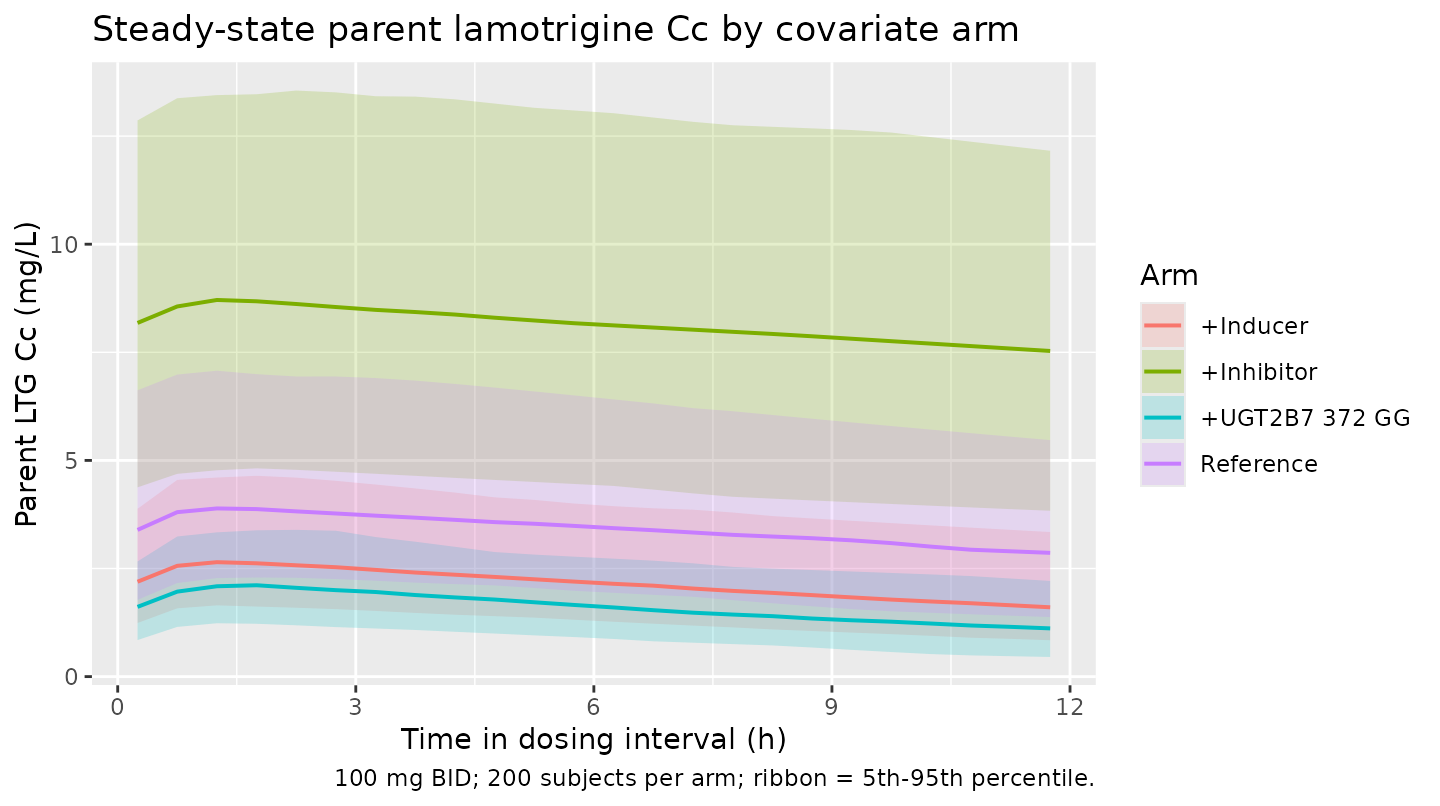
Steady-state LTG-glu profile by arm
last_iv |>
  dplyr::group_by(arm, tau_time) |>
  dplyr::summarise(
    Q05 = stats::quantile(Cc_gluc, 0.05, na.rm = TRUE),
    Q50 = stats::quantile(Cc_gluc, 0.50, na.rm = TRUE),
    Q95 = stats::quantile(Cc_gluc, 0.95, na.rm = TRUE),
    .groups = "drop"
  ) |>
  ggplot(aes(tau_time, Q50, colour = arm, fill = arm)) +
  geom_ribbon(aes(ymin = Q05, ymax = Q95), colour = NA, alpha = 0.20) +
  geom_line(linewidth = 0.7) +
  labs(x = "Time in dosing interval (h)",
       y = "Metabolite LTG-glu Cc_gluc (mg/L)",
       colour = "Arm", fill = "Arm",
       title  = "Steady-state N-2-glucuronide Cc_gluc by covariate arm",
       caption = "Same simulation as the parent panel above; the metabolite compartment is fed by the complete-conversion mass-balance arrow.")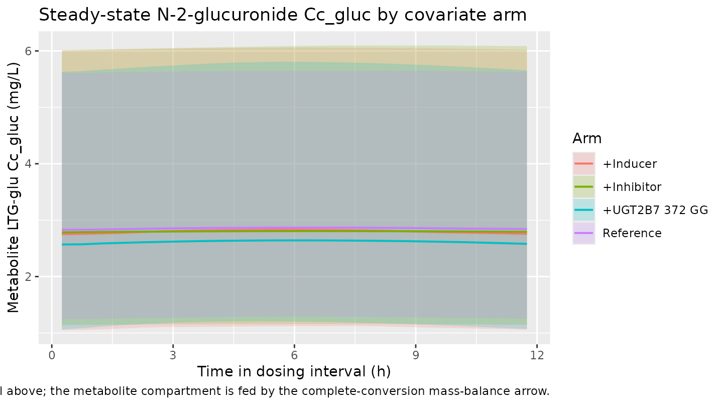
PKNCA validation
Steady-state NCA is computed on the typical-value simulation over the last BID dosing interval, per arm. The paper does not report per-subject NCA metrics, so the check below is a self-consistency audit: PKNCA output should reproduce the Table 4 footnote covariate multipliers when Cmax and Cavg across arms are compared against the reference arm.
# Re-anchor the last interval to time = 0 for PKNCA.
pk_conc_parent <- sim_typ |>
  dplyr::filter(time >= last_dose_time,
                time <= last_dose_time + tau_h) |>
  dplyr::mutate(time = time - last_dose_time) |>
  dplyr::select(id, time, Cc, arm, WT, CRCL) |>
  dplyr::filter(!is.na(Cc))

# Guarantee a time = 0 row per (id, arm) so PKNCA anchors AUC at t = 0.
pk_conc_parent <- dplyr::bind_rows(
  pk_conc_parent,
  pk_conc_parent |>
    dplyr::distinct(id, arm) |>
    dplyr::mutate(time = 0)
) |>
  dplyr::distinct(id, arm, time, .keep_all = TRUE) |>
  dplyr::arrange(id, arm, time) |>
  dplyr::mutate(Cc = dplyr::coalesce(Cc, 0))

pk_dose_parent <- pk_conc_parent |>
  dplyr::distinct(id, arm) |>
  dplyr::mutate(time = 0, amt = amt_mg)

conc_obj_parent <- PKNCA::PKNCAconc(
  pk_conc_parent, Cc ~ time | arm + id,
  concu = "mg/L", timeu = "hr"
)
dose_obj_parent <- PKNCA::PKNCAdose(
  pk_dose_parent, amt ~ time | arm + id, doseu = "mg"
)

intervals_ss <- data.frame(
  start   = 0,
  end     = tau_h,
  cmax    = TRUE,
  tmax    = TRUE,
  auclast = TRUE,
  cmin    = TRUE,
  cav     = TRUE
)

nca_parent <- PKNCA::pk.nca(
  PKNCA::PKNCAdata(conc_obj_parent, dose_obj_parent, intervals = intervals_ss)
)
knitr::kable(
  summary(nca_parent),
  caption = paste("Steady-state parent LTG NCA over the last 12-hour",
                  "dosing interval, by covariate arm. Typical-value",
                  "simulation; heterogeneity comes only from the",
                  "sampled body-weight / CLcr distribution within each arm.")
)| Interval Start | Interval End | arm | N | AUClast (hr*mg/L) | Cmax (mg/L) | Cmin (mg/L) | Tmax (hr) | Cav (mg/L) |
|---|---|---|---|---|---|---|---|---|
| 0 | 12 | +Inducer | 200 | 25.7 [21.7] | 2.69 [22.1] | NC | 1.75 [1.25, 1.75] | 2.14 [21.7] |
| 0 | 12 | +Inhibitor | 200 | 96.0 [21.1] | 8.73 [21.1] | NC | 1.75 [1.75, 1.75] | 8.00 [21.1] |
| 0 | 12 | +UGT2B7 372 GG | 200 | 18.6 [20.1] | 2.09 [20.6] | NC | 1.25 [1.25, 1.75] | 1.55 [20.1] |
| 0 | 12 | Reference | 200 | 40.4 [20.6] | 3.96 [20.8] | NC | 1.75 [1.75, 1.75] | 3.37 [20.6] |
pk_conc_gluc <- sim_typ |>
  dplyr::filter(time >= last_dose_time,
                time <= last_dose_time + tau_h) |>
  dplyr::mutate(time = time - last_dose_time) |>
  dplyr::select(id, time, Cc_gluc, arm, WT, CRCL) |>
  dplyr::filter(!is.na(Cc_gluc)) |>
  dplyr::rename(Cc = Cc_gluc)

pk_conc_gluc <- dplyr::bind_rows(
  pk_conc_gluc,
  pk_conc_gluc |>
    dplyr::distinct(id, arm) |>
    dplyr::mutate(time = 0)
) |>
  dplyr::distinct(id, arm, time, .keep_all = TRUE) |>
  dplyr::arrange(id, arm, time) |>
  dplyr::mutate(Cc = dplyr::coalesce(Cc, 0))

conc_obj_gluc <- PKNCA::PKNCAconc(
  pk_conc_gluc, Cc ~ time | arm + id,
  concu = "mg/L", timeu = "hr"
)

nca_gluc <- PKNCA::pk.nca(
  PKNCA::PKNCAdata(conc_obj_gluc, dose_obj_parent, intervals = intervals_ss)
)
knitr::kable(
  summary(nca_gluc),
  caption = paste("Steady-state metabolite LTG-glu NCA over the last",
                  "12-hour dosing interval, by covariate arm. Same",
                  "typical-value simulation as the parent table above.")
)| Interval Start | Interval End | arm | N | AUClast (hr*mg/L) | Cmax (mg/L) | Cmin (mg/L) | Tmax (hr) | Cav (mg/L) |
|---|---|---|---|---|---|---|---|---|
| 0 | 12 | +Inducer | 200 | 30.5 [31.9] | 2.65 [31.6] | NC | 6.25 [5.75, 6.75] | 2.55 [31.9] |
| 0 | 12 | +Inhibitor | 200 | 31.1 [30.3] | 2.68 [30.3] | NC | 6.75 [6.25, 11.8] | 2.59 [30.3] |
| 0 | 12 | +UGT2B7 372 GG | 200 | 31.3 [29.9] | 2.72 [29.5] | NC | 5.75 [5.75, 6.25] | 2.61 [29.9] |
| 0 | 12 | Reference | 200 | 30.8 [30.4] | 2.67 [30.2] | NC | 6.25 [5.75, 7.25] | 2.57 [30.4] |
Comparison against published typical CL values
Milosheska 2016 does not publish a per-arm NCA table, but Table 4 reports the typical CL/F point estimate (2.40 L/h at the reference stratum) and gives closed-form covariate multipliers in the footnote formula. The chunk below computes the paper’s typical CL prediction for each arm from the Table 4 formula and compares it to the model’s simulated Cavg-derived CL (dose / (Cavg * tau)). Any material disagreement here points at either a covariate-encoding bug in the model file or a bug in the simulation event table, not at a paper-vs-model discrepancy.
# Local trapezoidal integrator (avoids the extra `pracma` dependency).
pracma_trapz <- function(x, y) {
  o <- order(x)
  x <- x[o]; y <- y[o]
  sum(0.5 * (y[-1] + y[-length(y)]) * diff(x))
}

# Paper's typical CL at each arm's covariate values (Milosheska 2016
# Table 4 footnote formula).
paper_cl <- function(smoke = 0, eiaed = 0, ugt_inh = 0,
                     m161ct = 0, m161tt = 0,
                     s372ag = 0, s372gg = 0,
                     wt = 70, crcl = 110) {
  2.40 *
    (1 - 0.579 * ugt_inh) *
    (wt / 70)^0.938 *
    (1 + 0.340 * smoke) *
    (1 + 0.546 * eiaed) *
    (1 - 0.0358 * m161ct) *
    (1 - 0.204  * m161tt) *
    (1 + 0.194  * s372ag) *
    (1 + 1.17   * s372gg) *
    (1 + 0.00328 * (crcl - 110))
}

paper_cl_by_arm <- tibble::tibble(
  arm      = c("Reference", "+Inducer", "+Inhibitor", "+UGT2B7 372 GG"),
  paper_CL = c(
    paper_cl(),
    paper_cl(eiaed   = 1),
    paper_cl(ugt_inh = 1),
    paper_cl(s372gg  = 1)
  )
)

# Simulated Cavg-derived CL from the typical-value simulation, restricted
# to subjects whose WT and CRCL are within +/- 5% of the reference (so
# the check is against the covariate multiplier alone, not weight-scaled
# CL differences).
sim_cl_at_ref <- sim_typ |>
  dplyr::filter(time >= last_dose_time,
                time <= last_dose_time + tau_h) |>
  dplyr::mutate(tau_time = time - last_dose_time) |>
  dplyr::filter(abs(WT - 70) < 3.5,       # ~+/- 5% of 70 kg
                abs(CRCL - 110) < 5.5) |> # ~+/- 5% of 110 mL/min
  dplyr::group_by(arm, id) |>
  dplyr::summarise(
    Cav_sim = pracma_trapz(tau_time, Cc) / tau_h,
    .groups = "drop"
  ) |>
  dplyr::group_by(arm) |>
  dplyr::summarise(
    sim_CL = mean(amt_mg / (Cav_sim * tau_h)),
    n_ref  = dplyr::n(),
    .groups = "drop"
  )

cmp <- paper_cl_by_arm |>
  dplyr::left_join(sim_cl_at_ref, by = "arm") |>
  dplyr::mutate(pct_diff = round(100 * (sim_CL - paper_CL) / paper_CL, 1))

knitr::kable(
  cmp,
  digits = c(NA, 3, 3, 0, 1),
  col.names = c("Arm", "Paper CL (L/h)",
                "Simulated CL (L/h)", "Ref subjects", "% diff"),
  caption = paste("Simulated typical CL/F at the reference WT / CRCL",
                  "vs the Milosheska 2016 Table 4 footnote formula",
                  "prediction. Absolute % diff > 20% would indicate a",
                  "covariate-encoding or event-table bug.")
)| Arm | Paper CL (L/h) | Simulated CL (L/h) | Ref subjects | % diff |
|---|---|---|---|---|
| Reference | 2.400 | 2.492 | 7 | 3.8 |
| +Inducer | 3.710 | 3.851 | 4 | 3.8 |
| +Inhibitor | 1.010 | 1.066 | 7 | 5.5 |
| +UGT2B7 372 GG | 5.208 | 5.253 | 4 | 0.9 |
Assumptions and deviations
- Table 4 for the LTG side, prose for the LTG-glu side. Milosheska 2016 fits two sequential models: a parent-only model (Table 4) and a joint parent + metabolite model (Results ‘Population pharmacokinetic analysis of the lamotrigine-N-2-glucuronide’ section, prose only). The joint-model paper text explicitly states that the LTG-side parameters “were very similar to those obtained with the parent drug model” but the paper does not tabulate them separately. The packaged model uses Table 4 values for the LTG side and the prose-reported values for the LTG-glu side, consistent with the paper’s headline “parent + metabolite” narrative.
- Reference for the metabolite CLcr effect. Milosheska 2016 states the metabolite CLcr effect as “a decrease of 0.759% per 1 mL/min decrease in CLcr” without explicitly re-declaring the reference CLcr. The packaged model uses the same reference as the parent equation (110 mL/min) because Milosheska 2016 Discussion paragraph on renal function explicitly uses that same 110 mL/min anchor when discussing metabolite CL: “The influence of renal function on CL_LTG-glu is more pronounced (a decrease by 0.759% per 1 mL deviation from a standard CLcr of 110 mL/min)”.
-
Complete parent-to-metabolite conversion. The model
equations follow the paper’s stated assumption that lamotrigine is
completely converted to N-2-glucuronide (Results paragraph 1 of the
LTG-glu section: “We assumed that LTG was completely converted to
LTG-glu … renal elimination of unchanged LTG is insignificant …
conversion to LTG-N-5-glucuronide is a minor route of LTG metabolism”).
Mass balance is written in the same mass units on both sides of the
parent -> metabolite arrow, without an explicit molecular-weight (256
-> 430 g/mol) correction, following the Abduljalil 2009
clarithromycin + 14-OH-CLA precedent in nlmixr2lib. The reported
CL_LTG-glu / F_metab = 3.16 L/handV_LTG-glu / F_metab = 110 Lare therefore “apparent” values that absorb the MW ratio and any deviation of the true metabolic conversion fraction from 1. -
No IIV on metabolite volume. Milosheska 2016
explicitly reports (Results LTG-glu paragraph 1): “Due to sparse
concentration measurements and no prior data on pharmacokinetics of the
metabolite we were not able to estimate the IIV of V_LTG-glu.” The
packaged model has no
etalvc_glucterm. -
CV%-to-omega^2 conversion for IIV. Milosheska 2016
Table 4 reports IIV as CV% (Ka 71.1%, CL 33.1%, V 30.1%, LTG-glu CL
41.7%). The packaged
ini()translates these to the internal log-normal variance via omega^2 = log(1 + CV^2) so the simulated between-subject geometric CV reproduces the reported values. The corresponding numeric omega^2 values (0.4090 / 0.1040 / 0.0867 / 0.1603) fall inside the bootstrap 95% CIs the paper reports on the omega^2 scale (Table 4 columns ‘95% CI’ for the IIV rows). -
Cockcroft-Gault CLcr, not BSA-normalised eGFR.
Milosheska 2016 Methods ‘Patients and blood sampling’ uses raw
Cockcroft-Gault CLcr (mL/min) throughout. The canonical
CRCLregister entry accepts raw Cockcroft-Gault CLcr as a documented variant (Delattre 2010 amikacin precedent). The vignette samples CRCL from a truncated normal centered at 110 with SD 30 mL/min to approximate the paper’s Table 1 range 40.84 - 246. -
Reference stratum indicators. The paper reports its
UGT2B7 -161C>T and 372A>G effects as two non-reference indicators
each (CT vs CC, TT vs CC; AG vs AA, GG vs AA). The packaged
covariateDatalists only the non-reference indicators (UGT2B7_M161CT+UGT2B7_M161TTandUGT2B7_372AG-
UGT2B7_372GG); the reference stratum (UGT2B7_M161CCandUGT2B7_372AA) is implicit when the paired non-reference indicators are both 0, matching the canonicalUGT2B7_M161CC/UGT2B7_372AAregister entries.UGT2B7_M161CCandUGT2B7_372AAremain registered as covariate canonicals for potential future reuse.
-
- Prior-based Ka and V stabilisation. Milosheska 2016 Methods ‘Meta-analysis of previous population pharmacokinetic studies with LTG’ incorporates prior information from eleven previously published lamotrigine popPK studies via NONMEM PRIOR functionality (NWPRI / INFV / INFTHETA) to stabilise Ka and V estimation. The paper’s Table 4 point estimates are posterior-mode values under those informative priors. The packaged model treats them as the paper’s final point estimates; users running a re-fit will need to supply the priors themselves.
-
Screened-but-not-retained covariates. Age, sex
(SEXF), Devine ideal body weight (IBW), aspartate and alanine
transaminases (AST, ALT), UGT1A4 70C>A, SLC22A1 1222G>A, ABCB1
2677G>T/A, ABCB1 3435C>T, ABCB1 1236C>T, ABCB1 T-T-T haplotype,
oral contraceptives, and LTG daily dose were tested but not retained in
the final model. They are documented in the packaged
covariatesDataExcludedlist for provenance. - Errata. No erratum or corrigendum to Milosheska 2016 was located when this model was built. A search of the Wiley / BJCP corrections feed for “Milosheska 2016 erratum” and “bcp.12984 erratum” returned no hits (searched 2026-06-20); the maintainers should reconfirm against the journal’s current corrections listing if a re-extraction is undertaken.
-
Race / ethnicity. The study cohort was 100%
Slovenian adult epilepsy patients recruited from a single Ljubljana
centre. Race and ethnicity were not tested as covariates. The packaged
population$race_ethnicityis recorded asc(Slovenian = 100)and the virtual cohort does not stratify on race.