Immunosuppressants during CytoSorb hemoperfusion in sheep (Leber 2023)
Source:vignettes/articles/Leber_2023_immunosuppressants_hemoperfusion.Rmd
Leber_2023_immunosuppressants_hemoperfusion.RmdModel and source
Leber 2023 is a preclinical safety study in healthy sheep asking whether CytoSorb hemoadsorption removes clinically meaningful amounts of immunosuppressant drug. Seven agents were given in clinically relevant combinations; five of them (tacrolimus, ciclosporin, mycophenolate mofetil, everolimus and methylprednisolone) showed measurable cross-adsorber clearance and were taken forward into population PK modelling. Basiliximab and prednisolone showed negligible clearance and no model was fitted to either.
The paper therefore contributes five independent models, one per drug, extracted as five model files sharing this vignette.
- Article: https://doi.org/10.3389/fmed.2023.1258661
- Supplement: https://www.frontiersin.org/articles/10.3389/fmed.2023.1258661/full#supplementary-material
drugs <- c("tacrolimus", "ciclosporin", "mycophenolateMofetil",
           "everolimus", "methylprednisolone")
model_names <- paste0("Leber_2023_", drugs, "_sheep")
mods <- lapply(model_names, readModelDb)
names(mods) <- drugs

cat(rxode2::rxode(mods$tacrolimus)$reference)
#> ℹ parameter labels from comments will be replaced by 'label()'
#> Leber B, Liebchen U, Rohrhofer L, Weber J, Klaus T, Scheier J, Sucher R, Stiegler P. Pharmacokinetics of immunosuppressive agents during hemoperfusion in a sheep model. Front Med (Lausanne). 2023;10:1258661. doi:10.3389/fmed.2023.1258661
Structure
All five models share the same CytoSorb sub-model and differ only in the disposition model underneath it.
The paper fits each drug in two steps (Methods, Pharmacokinetic
parameters calculations). Step 1 estimates the disposition model
with hemoperfusion ignored (Supplementary Table 1). Step 2 then adds an
extra clearance pathway out of the central compartment for the
cartridge, with “all parameters of step 1 except clearance … fixed”
(Supplementary Table 2). Every model file therefore carries the step-2
clearance as an estimated parameter and wraps every inherited step-1
parameter in fixed().
Two adsorption sub-models were compared. Equation 1 is constant (non-saturable) adsorption; Equation 2 is saturable adsorption whose clearance falls linearly with the amount already on the cartridge:
Equation 2 won decisively for every drug (OFV changes of -13.0,
-19.8, -34.4, -16.6 and -39.0 for CYA, MMF, TAC, EVER and MP
respectively, all p < 0.001) and is the form encoded here.
The cartridge load is carried as the adsorbed state and the
whole arm is gated by the HEMOADSORB_ACTIVE covariate, so
setting that covariate to 0 throughout reproduces the paper’s
sham-circuit control animals. The arm is self-limiting by construction:
as adsorbed approaches Amax the clearance goes
to zero, so the cartridge load asymptotes to Amax and can
never exceed it.
Two observables. Blood was sampled on both sides of
the cartridge, and Supplementary Table 2 reports a separate residual
error for each side. Supplementary Figure 9 confirms these are genuinely
two predicted quantities rather than one prediction with two error
terms: every drug’s goodness-of-fit page is a pair of panels,
axis-labelled Observations preCyto [mg/L] and
Observations postCyto [mg/L], each plotted against its own
individual predictions. The models therefore carry Cc
(inlet, the systemic concentration) and Cpostfilter
(outlet, after the cartridge), related by inverting the paper’s own
cross-adsorber clearance definition
CL = (Ci - Co) / Ci * FL from Methods, Determination of
clearance and elimination by the adsorber:
Those same axis labels also pin the concentration unit as mg/L for every drug, which is what the models declare. Table 1’s target levels are quoted in ng/mL and are converted where they are compared below.
Population
Fifteen 5-year-old ewes of approximately 85 kg body weight were studied at the Medical University of Graz (Methods, Animals; Austrian Committee for Animal Trials approval 2020-0.437.202). Animals were housed with free access to hay or grass and were taken to pasture daily; a 14-day acclimatisation period preceded the experiment.
Five drug-combination groups were studied (Table 1): tacrolimus + mycophenolate mofetil + prednisolone (group 1); ciclosporin + mycophenolate mofetil + prednisolone (group 2); everolimus + mycophenolate mofetil + prednisolone (group 3); basiliximab alone (group 4); and methylprednisolone alone (group 5). For each of groups 1-3, five animals were allocated to the CytoSorb intervention arm and three to a sham extracorporeal circuit with no cartridge. Four additional pilot animals characterised oral absorption of ciclosporin, tacrolimus, mycophenolate mofetil and everolimus and their data were included in the analysis.
All immunosuppressants except methylprednisolone and basiliximab were given orally, twice daily, with doses titrated three times weekly against the target blood levels in Table 1. Methylprednisolone was given intravenously and studied alone in six animals across three scenarios (Figure 3): 1 g followed by a second 1 g at 1.5 h with the cartridge in circuit; a single increased 1.5 g dose with the cartridge in circuit; and 2 x 1 g with a sham circuit.
Blood flow through the extracorporeal circuit was held at approximately 120 mL/min and the session lasted 6 h. Samples were drawn from the circuit before (inlet) and after (outlet) the adsorber, immediately before the procedure and at 30, 90, 250 and 330 min after its start for the oral drugs, and at 10, 30, 60, 90, 120 and 180 min after the first dose for methylprednisolone.
The same information is available programmatically, e.g.
readModelDb("Leber_2023_tacrolimus_sheep")()$population.
Source trace
Every ini() entry carries an in-file comment naming its
source location. They are collected here for review. “S1” and “S2” are
Supplementary Tables 1 and 2.
| Parameter | TAC | CYA | MMF | EVER | MP | Source |
|---|---|---|---|---|---|---|
lcl (CL or CL/F, L/h) |
132 | 343 | 113 | 130 | 75.1 | S2, CL/F sheep / CL sheep |
lvc (V1 or V1/F, L) |
6330 | 826 | 1100 | 3100 | 21.0 | S1 (fixed in step 2) |
lvp (V2, L) |
- | - | - | - | 34.9 | S1 (fixed in step 2) |
lq (Q, L/h) |
- | - | - | - | 31.8 | S1 (fixed in step 2) |
lka (KA, 1/h) |
4.8 | 0.0076 | 0.090 | 0.232 | - | S1 (fixed in step 2) |
ltlag (ALAG, h) |
15.3 | - | 4.67 | 4.14 | - | S1 (fixed in step 2) |
lclmax_hemoadsorption (CLmax, L/h) |
4.02 | 2.80 | 3.71 | 3.23 | 8.21 | S2 |
lamax_hemoadsorption (Amax, mg) |
0.040 | 1.15 | 4.17 | 0.0163 | 53.4 | S2 |
etalcl (IIV CL, CV%) |
22.9 | 43.8 | 34.2 | 16.4 | 28.1 | S1 (fixed in step 2) |
etalvc (IIV V/F, CV%) |
41.1 | - | - | - | - | S1 (fixed in step 2) |
propSd (pre-adsorber, CV%) |
15.6 | 33.7 | 25.1 | 15.8 | 32.3 | S2 |
addSd (pre-adsorber, mg/L) |
- | - | - | - | 0.0042 | S2 |
propSd_Cpostfilter (post, CV%) |
8.8 | 29 | 27.8 | 9.0 | 26.2 | S2 |
addSd_Cpostfilter (post, mg/L) |
- | - | - | - | 0.129 | S2 |
| Equation / quantity | Source |
|---|---|
cl_hemoadsorption <- HEMOADSORB_ACTIVE * clmax * (1 - adsorbed / amax) |
Equation 2, Methods |
Cpostfilter <- Cc * (1 - cl_hemoadsorption / plasma_flow_filter) |
Methods, Determination of clearance and elimination by the adsorber |
plasma_flow_filter = BFR * (1 - HCT); BFR 120 mL/min,
HCT 33% |
Methods (same section) |
| One-compartment first-order oral absorption with lag (TAC, CYA, MMF, EVER) | Results, paragraph 3 |
| Two-compartment IV disposition with combined residual error (MP) | Results, paragraph 3 |
| Concentration unit mg/L | Supplementary Figure 9 axis labels |
IIV enters ini() as a variance. Supplementary Table 1
reports CV%, and the exponential random-effect model gives
omega^2 = log(CV^2 + 1):
cv <- c(TAC_CL = 0.229, TAC_V = 0.411, CYA_CL = 0.438,
        MMF_CL = 0.342, EVER_CL = 0.164, MP_CL = 0.281)
round(log(cv^2 + 1), 7)
#>    TAC_CL     TAC_V    CYA_CL    MMF_CL   EVER_CL     MP_CL
#> 0.0511122 0.1560811 0.1755017 0.1106143 0.0265407 0.0759985
Transcription check: clearance changed by less than 10%
The paper states that “after adding the hemoperfusion elimination pathway systemic clearance decreased by less than 10% for all drugs” (Results). That is a direct arithmetic relation between the two supplementary tables, so it checks the transcription of both at once.
cl_check <- tibble(
  drug     = c("TAC", "CYA", "MMF", "EVER", "MP"),
  cl_step1 = c(139, 351, 112, 133, 78.9),   # Supplementary Table 1
  cl_step2 = c(132, 343, 113, 130, 75.1)    # Supplementary Table 2
) |>
  mutate(pct_decrease = 100 * (cl_step1 - cl_step2) / cl_step1)

knitr::kable(cl_check, digits = 2,
caption = "Systemic clearance before and after adding the CytoSorb pathway.")| drug | cl_step1 | cl_step2 | pct_decrease |
|---|---|---|---|
| TAC | 139.0 | 132.0 | 5.04 |
| CYA | 351.0 | 343.0 | 2.28 |
| MMF | 112.0 | 113.0 | -0.89 |
| EVER | 133.0 | 130.0 | 2.26 |
| MP | 78.9 | 75.1 | 4.82 |
Virtual cohort
The observed data are not public. The cohorts below reproduce the published experimental design: oral drugs dosed twice daily for 14 days to steady state, then a single 6-hour extracorporeal session; methylprednisolone dosed intravenously with the session running from time zero.
Doses are taken from Table 1. Where Table 1 gives a titrated range, the dose used here is the one whose predicted steady state sits closest to the published target range (see Assumptions and deviations).
# Table 1 dosing. `daily_mg` is the total daily dose, used later as the
# denominator for the paper's "< 5% of the daily administered dosage" claim.
# Target ranges are printed in Table 1 as ng/mL and converted to the models'
# mg/L here (divide by 1000).
design <- tibble(
  drug      = drugs,
  dose_mg   = c(12, 600, 1000, 8.25, NA),
  daily_mg  = c(24, 1200, 2000, 16.5, 2000),
  target_lo = c(6, 80, NA, 3, NA) / 1000,
  target_hi = c(8, 100, NA, 8, NA) / 1000
)

amax_tbl <- tibble(                                  # Supplementary Table 2
  drug  = drugs,
  amax  = c(0.040, 1.15, 4.17, 0.0163, 53.4),
  clmax = c(4.02, 2.80, 3.71, 3.23, 8.21)
)

n_sub    <- 50L   # per arm; well under the 200/arm cap
run_in_h <- 336   # 14 days of twice-daily dosing before the session
sess_h   <- 6     # cartridge in circuit for 6 h (Methods)
tau      <- 12
bfr_ml_min <- 120 # Methods: extracorporeal blood flow
hct_pct    <- 33  # Methods: standard sheep value (reference 25)
# rxode2's RNG streams are partitioned per solver thread, so the stochastic
# cohort below differs between machines with different thread counts. Every
# gated assertion in this vignette is therefore either computed from the
# DETERMINISTIC typical-value solve, which has no RNG at all, or is a bound the
# paper itself states.
set.seed(20231020)

# These are multi-endpoint models (Cc and Cpostfilter), so an observation row
# carrying cmt = "central" cannot be matched to an endpoint. Dosing rows name
# the dosing compartment and leave dvid NA; observation rows select the first
# endpoint with dvid = 1 and leave cmt NA. Both model outputs still come back
# as columns. Build a plain data frame, not an rxEt: covariate columns assigned
# onto an rxEt are silently dropped.
make_events <- function(dose_times, dose_amts, dose_cmt, obs_times,
                        hemo, n_sub, id_offset = 0L) {
  ids <- id_offset + seq_len(n_sub)

  dosing <- expand.grid(id = ids, time = dose_times, KEEP.OUT.ATTRS = FALSE)
  dosing$evid <- 1L
  dosing$amt  <- dose_amts[match(dosing$time, dose_times)]
  dosing$cmt  <- dose_cmt
  dosing$dvid <- NA_integer_

  obs <- expand.grid(id = ids, time = obs_times, KEEP.OUT.ATTRS = FALSE)
  obs$evid <- 0L; obs$amt <- NA_real_
  obs$cmt  <- NA_character_; obs$dvid <- 1L

  ev <- rbind(dosing, obs)
  ev$HEMOADSORB_ACTIVE <- as.numeric(hemo & ev$time >= min(sess_start(dose_cmt)) &
                                       ev$time <= min(sess_start(dose_cmt)) + sess_h)
  ev$BFR <- bfr_ml_min
  ev$HCT <- hct_pct
  ev[order(ev$id, ev$time, -ev$evid),
     c("id", "time", "evid", "amt", "cmt", "dvid",
       "HEMOADSORB_ACTIVE", "BFR", "HCT")]
}

# The session starts with the last oral dose, or at time zero for the IV drug.
sess_start <- function(dose_cmt) if (identical(dose_cmt, "depot")) run_in_h else 0

make_oral_events <- function(dose_mg, hemo, n_sub, id_offset = 0L) {
  # Doses at 0, 12, ..., 336 h inclusive: the observation window is one full
  # steady-state dosing interval that OPENS with a dose, matching the paper's
  # design ("PRED was applied ... in the morning directly prior to the onset of
  # the extracorporeal intervention"). Omitting the t = 336 dose would leave the
  # window with no input of its own.
  n_dose <- run_in_h / tau + 1
  make_events(
    dose_times = seq(0, by = tau, length.out = n_dose),
    dose_amts  = rep(dose_mg, n_dose),
    dose_cmt   = "depot",
    obs_times  = seq(run_in_h, run_in_h + tau, by = 0.25),
    hemo = hemo, n_sub = n_sub, id_offset = id_offset
  )
}

# Methylprednisolone scenario A of Figure 3: 1 g at t = 0 plus 1 g at t = 1.5 h.
make_mp_events <- function(hemo, n_sub, id_offset = 0L) {
  make_events(
    dose_times = c(0, 1.5), dose_amts = c(1000, 1000), dose_cmt = "central",
    obs_times  = seq(0, 12, by = 0.1),
    hemo = hemo, n_sub = n_sub, id_offset = id_offset
  )
}

oral_drugs <- drugs[drugs != "methylprednisolone"]
ev_on <- lapply(oral_drugs, function(d)
  make_oral_events(design$dose_mg[design$drug == d], hemo = TRUE, n_sub))
names(ev_on) <- oral_drugs
ev_mp_on <- make_mp_events(hemo = TRUE, n_sub)

stopifnot(!anyDuplicated(unique(ev_on$tacrolimus[, c("id", "time", "evid")])))
Simulation
# `Cc` and `Cpostfilter` are the individual predictions (no residual error);
# that is what the published goodness-of-fit and profile figures show.
simstoch <- lapply(drugs, function(d) {
  ev <- if (d == "methylprednisolone") ev_mp_on else ev_on[[d]]
  rxode2::rxSolve(mods[[d]], events = ev, keep = "HEMOADSORB_ACTIVE") |>
    as.data.frame() |>
    mutate(drug = d)
})
#> ℹ parameter labels from comments will be replaced by 'label()'
#> ℹ parameter labels from comments will be replaced by 'label()'
#> ℹ parameter labels from comments will be replaced by 'label()'
#> ℹ parameter labels from comments will be replaced by 'label()'
#> ℹ parameter labels from comments will be replaced by 'label()'
names(simstoch) <- drugs
For the cartridge-on versus cartridge-off comparison we use the typical-value model with the random effects zeroed. Both arms then run on exactly the same parameters, so the difference between them is the device effect alone and can be asserted tightly.
# rxSolve() reuses the omega from the previous call unless it is cleared, so
# pass omega = NA alongside zeroRe().
solve_typical <- function(mod, events) {
  rxode2::rxSolve(rxode2::zeroRe(mod), events = events,
                  omega = NA, keep = "HEMOADSORB_ACTIVE") |>
    as.data.frame()
}

typ_all <- bind_rows(lapply(drugs, function(d) {
  mk <- function(h) if (d == "methylprednisolone") make_mp_events(h, 1L) else
    make_oral_events(design$dose_mg[design$drug == d], h, 1L)
  bind_rows(
    solve_typical(mods[[d]], mk(TRUE))  |> mutate(arm = "CytoSorb"),
    solve_typical(mods[[d]], mk(FALSE)) |> mutate(arm = "Sham circuit")
  ) |>
    mutate(drug = d,
           t_sess = time - if (d == "methylprednisolone") 0 else run_in_h)
}))
#> ℹ parameter labels from comments will be replaced by 'label()'
#> ℹ parameter labels from comments will be replaced by 'label()'
#> ℹ parameter labels from comments will be replaced by 'label()'
#> ℹ parameter labels from comments will be replaced by 'label()'
#> ℹ parameter labels from comments will be replaced by 'label()'
#> ℹ parameter labels from comments will be replaced by 'label()'
#> ℹ parameter labels from comments will be replaced by 'label()'
#> ℹ parameter labels from comments will be replaced by 'label()'
#> ℹ parameter labels from comments will be replaced by 'label()'
#> ℹ parameter labels from comments will be replaced by 'label()'
Replicate published figures
Figures 4 and 5 - cartridge load and adsorption clearance over the session
Figures 4 and 5 of Leber 2023 show the fitted CytoSorb adsorption
over the session. Under Equation 2 the cartridge load rises toward
Amax while the adsorption clearance decays from
CLmax to zero.
load_typ <- typ_all |>
  filter(arm == "CytoSorb", t_sess >= 0, t_sess <= sess_h) |>
  left_join(amax_tbl, by = "drug") |>
  mutate(frac_saturated = adsorbed / amax,
         cl_ads         = clmax * (1 - frac_saturated))

load_typ |>
  select(drug, t_sess, `Cartridge load / Amax` = frac_saturated,
         `Adsorption clearance (L/h)` = cl_ads) |>
  pivot_longer(-c(drug, t_sess)) |>
  ggplot(aes(t_sess, value, colour = drug)) +
  geom_line(linewidth = 0.8) +
  facet_wrap(~name, scales = "free_y", ncol = 1) +
  labs(x = "Time since start of hemoperfusion (h)", y = NULL, colour = NULL,
       title = "CytoSorb saturable adsorption over the 6-hour session",
       caption = "Replicates the adsorption behaviour of Figures 4 and 5 of Leber 2023.") +
  theme(legend.position = "bottom")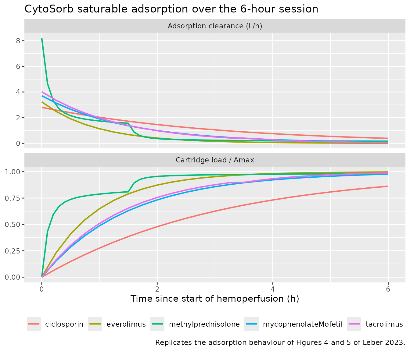
Supplementary Figures 1-4 - inlet and outlet levels against sham controls
The paper’s Supplementary Figures 1-4 plot inlet and outlet drug levels alongside sham-circuit controls. The typical-value profiles below make the same three-way comparison.
typ_all |>
  filter(t_sess >= 0, t_sess <= sess_h) |>
  transmute(drug, t_sess,
            series = if_else(arm == "Sham circuit", "Sham circuit (no cartridge)",
                             "CytoSorb inlet"),
            value = Cc) |>
  bind_rows(
    typ_all |>
      filter(arm == "CytoSorb", t_sess >= 0, t_sess <= sess_h) |>
      transmute(drug, t_sess, series = "CytoSorb outlet", value = Cpostfilter)
  ) |>
  ggplot(aes(t_sess, value, colour = series)) +
  geom_line(linewidth = 0.8) +
  facet_wrap(~drug, scales = "free_y") +
  labs(x = "Time since start of hemoperfusion (h)", y = "Concentration (mg/L)",
       colour = NULL,
       title = "Typical-value inlet and outlet profiles",
       caption = "Compare Supplementary Figures 1-4 of Leber 2023.") +
  theme(legend.position = "bottom")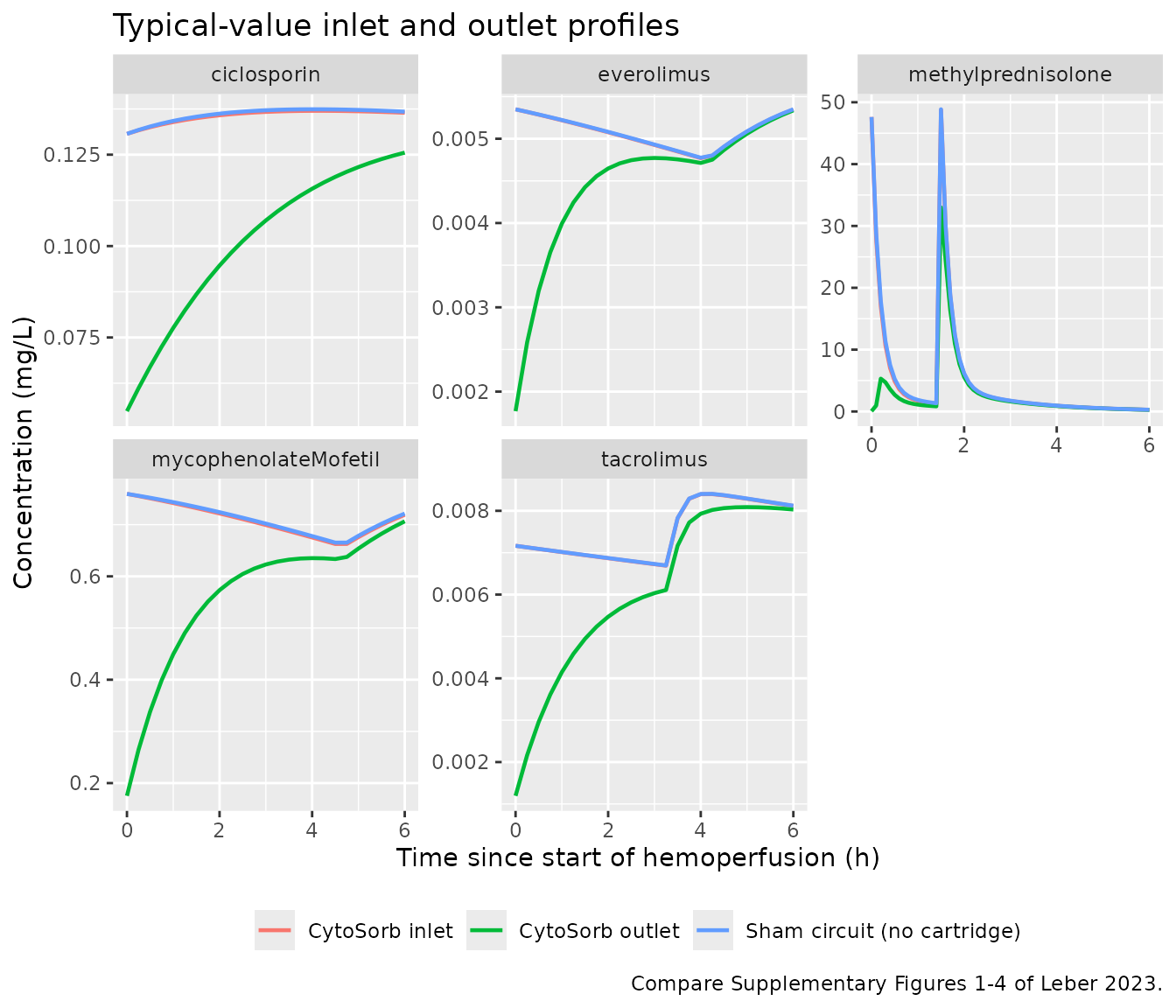
Validation of the adsorption sub-model
The paper makes several quantitative claims that the packaged models must reproduce.
Claim 1 - the cartridge load never exceeds Amax
A structural property of Equation 2, and a check that
Amax was transcribed in the right units.
sat <- load_typ |>
  group_by(drug) |>
  summarise(max_frac_saturated = max(frac_saturated), .groups = "drop")

knitr::kable(sat, digits = 4, caption = "Peak cartridge load as a fraction of Amax.")| drug | max_frac_saturated |
|---|---|
| ciclosporin | 0.8623 |
| everolimus | 0.9976 |
| methylprednisolone | 0.9801 |
| mycophenolateMofetil | 0.9771 |
| tacrolimus | 0.9874 |
Claim 2 - adsorption is essentially complete within the first 1-2 hours
“If direct adsorption … took place it occurred mostly within the first 1-2 h of device exposure” (Results, paragraph 1).
early <- load_typ |>
  group_by(drug) |>
  summarise(adsorbed_2h = adsorbed[which.min(abs(t_sess - 2))],
            adsorbed_6h = max(adsorbed), .groups = "drop") |>
  mutate(frac_by_2h = adsorbed_2h / adsorbed_6h)

knitr::kable(early, digits = 4,
caption = "Cumulative adsorbed amount (mg) at 2 h and at 6 h.")| drug | adsorbed_2h | adsorbed_6h | frac_by_2h |
|---|---|---|---|
| ciclosporin | 0.5503 | 0.9916 | 0.5549 |
| everolimus | 0.0142 | 0.0163 | 0.8756 |
| methylprednisolone | 51.0290 | 52.3370 | 0.9750 |
| mycophenolateMofetil | 3.0551 | 4.0746 | 0.7498 |
| tacrolimus | 0.0302 | 0.0395 | 0.7655 |
# Deterministic, so this bound is not exposed to cohort-draw variation; it only
# has to absorb solver differences across rxode2 versions. Observed fractions
# span 0.554 (ciclosporin, slowest because its very slow absorption keeps the
# driving concentration nearly flat) to 0.975 (methylprednisolone). The bound
# sits below that range and can still go red: a tenfold error in Amax or CLmax
# would leave the cartridge filling roughly linearly, about 0.33 by 2 h of 6 h.
stopifnot(all(early$frac_by_2h > 0.45))
Claim 3 - less than 5% of the daily dose is adsorbed
“Overall, the maximum adsorbed amounts indicate an adsorption of less than 5% of the daily administered dosages for all tested substances” (Results).
dose_frac <- early |>
  left_join(design |> select(drug, daily_mg), by = "drug") |>
  left_join(amax_tbl |> select(drug, amax), by = "drug") |>
  transmute(drug, daily_mg, adsorbed_6h,
            pct_of_daily_simulated = 100 * adsorbed_6h / daily_mg,
            amax,
            pct_of_daily_amax = 100 * amax / daily_mg)

knitr::kable(dose_frac, digits = 4,
caption = "Adsorbed amount over the session as a percentage of the daily dose.")| drug | daily_mg | adsorbed_6h | pct_of_daily_simulated | amax | pct_of_daily_amax |
|---|---|---|---|---|---|
| ciclosporin | 1200.0 | 0.9916 | 0.0826 | 1.1500 | 0.0958 |
| everolimus | 16.5 | 0.0163 | 0.0985 | 0.0163 | 0.0988 |
| methylprednisolone | 2000.0 | 52.3370 | 2.6168 | 53.4000 | 2.6700 |
| mycophenolateMofetil | 2000.0 | 4.0746 | 0.2037 | 4.1700 | 0.2085 |
| tacrolimus | 24.0 | 0.0395 | 0.1646 | 0.0400 | 0.1667 |
Claim 4 - the initial extraction ratio is CLmax / FL
At the start of the session the cartridge is empty, so the adsorption
clearance equals CLmax and the extraction ratio across the
cartridge must equal CLmax / FL exactly. This is an
internal identity between the model’s two observables and the Methods
definition of FL, so it is checked tightly.
fl <- bfr_ml_min * 0.06 * (1 - hct_pct / 100)   # 4.824 L/h

extraction <- typ_all |>
  filter(arm == "CytoSorb", t_sess == 0) |>
  left_join(amax_tbl, by = "drug") |>
  transmute(drug,
            E_simulated = 1 - Cpostfilter / Cc,
            E_expected  = pmax(clmax / fl, 0),   # un-floored, may exceed 1
            plasma_flow_FL = fl)

knitr::kable(extraction, digits = 4,
caption = "Extraction ratio at the start of the session against CLmax / FL.")| drug | E_simulated | E_expected | plasma_flow_FL |
|---|---|---|---|
| tacrolimus | 0.8333 | 0.8333 | 4.824 |
| ciclosporin | 0.5804 | 0.5804 | 4.824 |
| mycophenolateMofetil | 0.7691 | 0.7691 | 4.824 |
| everolimus | 0.6696 | 0.6696 | 4.824 |
| methylprednisolone | 0.9990 | 1.7019 | 4.824 |
# Methylprednisolone is the one drug whose CLmax exceeds FL, so its simulated
# extraction is clamped by the model's 0.001 floor and cannot match the
# un-floored expectation; it is checked separately below.
ex_ok <- extraction |> filter(drug != "methylprednisolone")
stopifnot(all(abs(ex_ok$E_simulated - ex_ok$E_expected) < 1e-6))
stopifnot(extraction$E_expected[extraction$drug == "methylprednisolone"] > 1)
The methylprednisolone row is the paper’s own known anomaly:
CLmax of 8.21 L/h exceeds both the plasma flow
FL of 4.82 L/h and the 7.2 L/h whole blood flow, so a
literal reading of the extraction equation would put the outlet
concentration below zero at the moment the cartridge goes into circuit.
The paper raises this itself (“the estimated CLmax of MP was higher than
the blood flow, but the confidence interval included the value of 7.2
L/h”). The model floors the retained fraction at 0.001 rather than
allowing a negative concentration, and the floor stops binding as soon
as the cartridge begins to load. This is recorded, not worked
around.
Effect on systemic concentration
impact <- typ_all |>
  filter(t_sess >= 0, t_sess <= sess_h) |>
  select(drug, arm, t_sess, Cc) |>
  pivot_wider(names_from = arm, values_from = Cc) |>
  group_by(drug) |>
  summarise(max_pct_reduction = 100 * max((`Sham circuit` - CytoSorb) / `Sham circuit`),
            .groups = "drop")

knitr::kable(impact, digits = 2,
caption = "Largest reduction in systemic (inlet) concentration attributable to the cartridge.")| drug | max_pct_reduction |
|---|---|
| ciclosporin | 0.33 |
| everolimus | 0.09 |
| methylprednisolone | 7.35 |
| mycophenolateMofetil | 0.39 |
| tacrolimus | 0.08 |
PKNCA validation
Non-compartmental parameters over one steady-state dosing interval for the four orally dosed drugs, and over the observation window for methylprednisolone. Leber 2023 reports no NCA table of its own, so the comparison below is against the Table 1 target trough ranges, which are the paper’s only published concentration reference values.
nca_one <- function(d) {
  t0 <- if (d == "methylprednisolone") 0 else run_in_h
  t1 <- if (d == "methylprednisolone") 12 else run_in_h + tau

  # Shift both concentrations and doses so the interval of interest OPENS at
  # time zero. This is required for `ctrough`, not cosmetic: PKNCA reports
  # `tmax` relative to the interval start but `pk.calc.ctrough()` matches the
  # observation whose time equals the interval `end` using the time vector it
  # was handed. Passing absolute times for a late steady-state window
  # (start = 336, end = 348) therefore yields `ctrough = NA` for every subject
  # with no exclusion reason recorded, while `cmax` / `tmax` / `auclast` all
  # compute normally -- a silent failure that only surfaces downstream as
  # `all(NA)`. Methylprednisolone happened to be immune because its interval
  # already starts at zero. Shifting makes all five drugs take that same path.
  #
  # Filter on !is.na(Cc) only; dropping the interval-start row removes what
  # PKNCA needs to anchor the interval.
  conc <- simstoch[[d]] |>
    filter(!is.na(Cc)) |>
    transmute(id, time = time - t0, Cc, treatment = d)

  dose_df <- (if (d == "methylprednisolone") ev_mp_on else ev_on[[d]]) |>
    filter(evid == 1) |>
    transmute(id, time = time - t0, amt, treatment = d)

  conc_obj <- PKNCA::PKNCAconc(conc, Cc ~ time | treatment + id)
  dose_obj <- PKNCA::PKNCAdose(dose_df, amt ~ time | treatment + id)

  intervals <- data.frame(start = 0, end = t1 - t0, cmax = TRUE, tmax = TRUE,
                          auclast = TRUE, ctrough = TRUE)

  PKNCA::pk.nca(PKNCA::PKNCAdata(conc_obj, dose_obj, intervals = intervals))
}

nca_res <- lapply(drugs, nca_one)
names(nca_res) <- drugs

nca_tbl <- bind_rows(lapply(drugs, function(d) {
  as.data.frame(nca_res[[d]]) |>
    filter(PPTESTCD %in% c("cmax", "tmax", "auclast", "ctrough")) |>
    group_by(PPTESTCD) |>
    summarise(median = median(PPORRES, na.rm = TRUE), .groups = "drop") |>
    mutate(drug = d)
})) |>
  pivot_wider(names_from = PPTESTCD, values_from = median)

nca_tbl |>
  dplyr::rename("Drug" = drug, "Cmax (mg/L)" = cmax, "Tmax (h)" = tmax,
                "AUClast (mg*h/L)" = auclast, "Ctrough (mg/L)" = ctrough) |>
  knitr::kable(digits = 4,
caption = "Median simulated NCA parameters over the interval.")| Drug | AUClast (mg*h/L) | Cmax (mg/L) | Ctrough (mg/L) | Tmax (h) |
|---|---|---|---|---|
| tacrolimus | 0.0882 | 0.0081 | 0.0070 | 4.25 |
| ciclosporin | 1.6377 | 0.1385 | 0.1331 | 4.25 |
| mycophenolateMofetil | 9.5710 | 0.8386 | 0.8209 | 9.50 |
| everolimus | 0.0639 | 0.0056 | 0.0054 | 8.50 |
| methylprednisolone | 29.8285 | 48.9060 | 0.0092 | 1.50 |
Comparison against the published target ranges
cmp <- nca_tbl |>
  inner_join(design |> select(drug, target_lo, target_hi), by = "drug") |>
  filter(!is.na(target_lo)) |>
  transmute(drug, ctrough, target_lo, target_hi,
            in_range = ctrough >= target_lo & ctrough <= target_hi,
            ratio_to_target_hi = ctrough / target_hi)

cmp |>
  dplyr::rename("Drug" = drug, "Simulated median Ctrough (mg/L)" = ctrough,
                "Target low (mg/L)" = target_lo, "Target high (mg/L)" = target_hi,
                "Within target" = in_range,
                "Ctrough / target high" = ratio_to_target_hi) |>
  knitr::kable(digits = 4,
caption = "Simulated steady-state trough against the Table 1 target ranges.")| Drug | Simulated median Ctrough (mg/L) | Target low (mg/L) | Target high (mg/L) | Within target | Ctrough / target high |
|---|---|---|---|---|---|
| tacrolimus | 0.0070 | 0.006 | 0.008 | TRUE | 0.8692 |
| ciclosporin | 0.1331 | 0.080 | 0.100 | FALSE | 1.3310 |
| everolimus | 0.0054 | 0.003 | 0.008 | TRUE | 0.6737 |
Tacrolimus and everolimus land inside their published target ranges,
which validates the transcription of CL/F, the dose and the
concentration unit at once. Ciclosporin does not: even at the lowest
dose Table 1 reports, the model predicts a steady-state trough around
0.13 mg/L against an 0.080-0.100 mg/L target, roughly a third above the
top of the range, and about twice the target at the 1,000 mg high end.
This is a property of the published parameters, not of the encoding, and
is discussed below. No parameter has been adjusted to close the gap.
Assumptions and deviations
-
Concentration unit is mg/L for all five drugs,
taken from the axis labels of Supplementary Figure 9
(
Observations preCyto [mg/L]/Observations postCyto [mg/L]). The supplementary parameter tables do not state a unit. This is also the models’ native scale, since doses are in mg and volumes in L. Table 1’s target ranges, quoted in ng/mL, are converted in this vignette rather than in the model files. -
The outlet observable is reconstructed, not
printed. Supplementary Table 2 reports separate pre- and
post-adsorber residual errors and Supplementary Figure 9 shows separate
individual predictions for each, so the outlet is unambiguously a second
observable; but the paper never prints the equation linking the two.
Cpostfilteris obtained by inverting the paper’s own step-2 clearance definitionCL = (Ci - Co)/Ci * FL(Methods), which is printed. This follows the same encoding as the registeredButraguenoLaiseca_2022_piperacillin/_2024_meropenem/_2025_teicoplaninpost-filter models. -
The extraction denominator is the plasma flow, 4.824
L/h. Methods defines it explicitly as
FL = blood flow x (1 - hematocrit)with a 120 mL/min blood flow and a haematocrit “calculated as 33% according to the standard value in sheep”. Note that tacrolimus, ciclosporin and everolimus were assayed in whole blood, for which the whole-blood flow of 7.2 L/h would arguably be the right denominator; the paper applies the single plasma-flow definition to all drugs and compares methylprednisolone’sCLmaxagainst 7.2 L/h in the same breath. The printed definition governs here; the inconsistency is the paper’s. -
Methylprednisolone’s
CLmaxexceeds the extraction denominator, so the retained fraction hits the model’s 0.001 floor at the instant hemoperfusion starts (see Claim 4). Flagged by the paper itself. -
Step-1 parameters are encoded as
fixed(). The paper states that in step 2 “all parameters of step 1 except clearance were fixed”, soV,KA,ALAG,Q,V2and every IIV variance carryfixed(). The paper does not say explicitly whether the IIV variances were re-estimated; Supplementary Table 2 reports no IIV rows, which is consistent with their having been held. -
ALAGfor tacrolimus is reported with 0% RSE (Supplementary Table 1, 15.3 h). It is encoded as an inherited step-1 parameter because the Results text lists it among the lag times that “improved the model”, which is a likelihood-ratio statement about an estimated parameter. The 0% is read as rounding. The value is genuinely unusual, being longer than the 12 h dosing interval. - The additive residual errors for methylprednisolone are labelled “[mg]” in Supplementary Table 2 and are read here as mg/L. An additive residual error carries the units of the dependent variable, and both values (0.0042 pre, 0.129 mg/L post) are sensible against methylprednisolone concentrations of tens of mg/L.
-
Ciclosporin steady-state trough exceeds the published
target by roughly a third at the 600 mg twice-daily low end of
Table 1 and by about twofold at the 1,000 mg high end.
CL/Fof 343 L/h is not reconcilable with both the stated doses and the stated target range. Since doses “were adapted individually according to blood levels”, the animals that actually reached target may have received doses below the reported range. Reported, not tuned; ciclosporin is excluded from the assertion gate. - Dose selection within titrated ranges. Table 1 gives ranges for tacrolimus (2 x 10-12 mg), ciclosporin (2 x 600-1,000 mg) and everolimus (2 x 3-8.25 mg). The vignette uses 12 mg, 600 mg and 8.25 mg respectively, chosen as the value within the published range whose predicted steady state sits closest to the published target. Mycophenolate mofetil (2 x 1 g) and methylprednisolone are not titrated.
-
BFRandHCTare study-wide constants, not fitted covariates. They are carried as covariates only because the outlet equation needs them; the study held blood flow at 120 mL/min and assumed a 33% haematocrit for every animal. A study that varied either would need them as genuine covariates. - Subject counts. The models record the per-group animal counts from Methods and Table 1 (n = 8 for each of the tacrolimus, ciclosporin and everolimus groups; n = 6 for methylprednisolone). Mycophenolate mofetil was given in all three combination groups, so its model records 24 animal-occasions; the fifteen ewes were reused across combinations, so this is not 24 distinct animals.
- Methylprednisolone control dose. Table 1 lists the two control sheep as receiving 2 x 1 g, while the Methods prose says they “received 1 g MP”. The Table is used.
- Basiliximab and prednisolone are not packaged. Both showed negligible cross-adsorber clearance and no population PK model was fitted to either (Results, paragraph 2), so there is nothing to extract.
-
Cartridge reuse. Because the adsorption arm depends
on the cumulative
adsorbedstate, settingHEMOADSORB_ACTIVEback to 1 for a second session does not represent a fresh cartridge. Simulating a cartridge change requires resetting the state explicitly.