Efavirenz (Vucicevic 2025)
Source:vignettes/articles/Vucicevic_2025_efavirenz.Rmd
Vucicevic_2025_efavirenz.RmdModel and source
mod <- rxode2::rxode2(readModelDb("Vucicevic_2025_efavirenz"))
#> ℹ parameter labels from comments will be replaced by 'label()'- Citation: Vucicevic K, Michalickova D, Obradovic B, Ranin J, Jevtovic D, Lukic R, Owen A, Dragovic G. Population pharmacokinetic-pharmacogenetic (PopPK-PGx) model of efavirenz in HIV-1-infected patients. Cureus. 2025;17(7):e88533. doi:10.7759/cureus.88533.
- Description: One-compartment population pharmacokinetic-pharmacogenetic (PopPK-PGx) model for oral efavirenz in Caucasian HIV-1-infected adults (Vucicevic 2025), with binary CYP2B6 c.516G>T (rs3745274) carrier and CYP2B6 c.485-18C>T (rs4803419) TT-homozygote effects on apparent oral clearance CL/F. Absorption rate ka and apparent volume V/F were not estimable from the one-sample-per-patient sparse design and are fixed to literature values (0.3 1/h and 237 L).
- Article: https://doi.org/10.7759/cureus.88533
Vucicevic 2025 is a population pharmacokinetic-pharmacogenetic (PopPK-PGx) re-analysis of a Serbian cohort of adults with HIV-1 who were previously reported in a single-timepoint concentration study (Olagunju 2014, the paper’s reference 17). The analysis quantifies the effect of two CYP2B6 polymorphisms on apparent oral efavirenz clearance and then uses the fitted model to simulate the probability of achieving the 1,000-4,000 ng/mL therapeutic window under different pharmacogenetic backgrounds and different non-adherence patterns.
Population
pop <- mod$populationThe analysis dataset comprised 89 adults with confirmed HIV-1 infection, all of white Caucasian ethnicity, receiving 600 mg efavirenz once daily as part of efavirenz-based antiretroviral therapy for at least three months (Methods, “PopPK-PGx model development”). Median body weight was 76 kg (IQR 66-85) and median age 40 years (IQR 32-48); 67.4% were smokers (Table 1). Patients on concomitant antituberculosis medication or other drugs known to interact with efavirenz metabolism, patients under 18 years, and pregnant women were excluded.
The design is extremely sparse: exactly one steady-state plasma sample per patient, drawn between 2.83 and 13.42 h after the last dose (Results paragraph 1; Appendix 1 Figure 4). That single-sample design is the reason the absorption rate constant and the apparent volume of distribution could not be estimated and were fixed to literature values.
Genotype frequencies in the cohort (Table 1):
| Polymorphism | Flagged n (%) | Retained in final model |
|---|---|---|
| CYP2B6 c.516G>T (rs3745274) | 30 (33.71) | Yes |
| CYP2B6 c.485-18C>T (rs4803419) | 12 (13.48) | Yes |
| NR1I3 c.540C>T (rs2307424) | 53 (59.60) | No |
| NR1I3 c.152-1089T>C (rs3003596) | 58 (65.17) | No |
Neither NR1I3 polymorphism showed a detectable effect on
efavirenz CL/F (Discussion paragraph 4); both are recorded in the model
file’s covariatesDataExcluded metadata together with the
demographic covariates that were screened but not retained.
Source trace
Every value in the model file, and where it comes from.
| Item | Value | Source location |
|---|---|---|
| Structural model | One compartment, first-order absorption and elimination (ADVAN2 TRANS2) | Methods, ‘PopPK-PGx model development’ paragraph 3 |
| ka | 0.3 1/h (fixed) | Methods paragraph 3 and Discussion paragraph 2 (cited to reference 20, Csajka 2003) |
| V/F | 237 L (fixed) | Methods paragraph 3 and Discussion paragraph 2 (‘237 L/70 kg’, references 9, 11, 18, 19) |
| CL/F (CLp) | 13.9 L/h (RSE 4%) | Table 2, row CLp (bootstrap 13.9; 95% CI 12.73-15.21) |
| CL/F covariate equation | CL/F = CLp * (1 + theta_RSA)^RSA * (1 + theta_RSB)^RSB | Table 2, header row of the ‘Fixed effects’ block |
| theta_RSA (CYP2B6 516G>T carrier) | -0.364 (RSE 14%) | Table 2, row theta_RSA (bootstrap -0.368; 95% CI -0.457 to -0.255) |
| theta_RSB (CYP2B6 c.485-18C>T TT) | -0.268 (RSE 16%) | Table 2, row theta_RSB (no bootstrap value reported) |
| IIV on CL/F | CV 13.1% (RSE 35%), exponential / log-normal | Table 2, row CV CL (%); Results paragraph 2 (bootstrap 13.4%; 95% CI 3.24-20.9%) |
| Residual error | Proportional, SD 0.25 (RSE 11%) | Table 2, row Proportional error; Results paragraph 2 (bootstrap 0.244; 95% CI 0.182-0.299) |
| RSA definition | Binary carrier indicator for CYP2B6 516G>T | Table 2 footnote |
| RSB definition | Binary indicator, CYP2B6 c.485-18C>T TT genotype | Table 2 footnote (called ‘carrier’), resolved to TT by Results paragraph 2 and the Table 3 row labels |
| Dosing regimen simulated | 600 mg once daily | Methods, ‘Model-based dose simulations’ |
| Therapeutic window | 1,000-4,000 ng/mL | Methods, ‘Model-based dose simulations’; Results, ‘Model-derived dosing implications’ |
| Reference Ctrough by genotype | 1,179.4 / 1,757.15 / 2,140.05 / 3,072.75 ng/mL | Table 3, column ‘Median C trough (95% CI)’ |
The ini() block reproduces
CL/F = CLp * (1 + theta_RSA)^RSA * (1 + theta_RSB)^RSB
literally. Because RSA and RSB are 0/1
indicators, each factor collapses to 1 when its indicator is 0. The
canonical covariate columns are 0/1/2 allele counts, from which
model() recovers the paper’s indicators as
RSA = (SNP_CYP2B6_RS3745274_T_COUNT >= 1) (dominant /
carrier model) and
RSB = (SNP_CYP2B6_RS4803419_T_COUNT == 2) (recessive /
TT-only model).
Virtual cohort
Table 3 of the paper simulates four genotype combinations at the standard 600 mg once-daily regimen. We reproduce the same four arms, each with 200 virtual subjects carrying inter-individual variability on CL/F.
tau        <- 24     # dosing interval (h)
n_doses    <- 21     # dose at t = 0, 24, ..., 480 -- >= 19 half-lives for the slowest arm
dose_mg    <- 600
n_per_arm  <- 200
t_last     <- tau * (n_doses - 1)

genotypes <- tibble::tribble(
  ~treatment,                     ~rs3745274_T, ~rs4803419_T,
  "516GG, c.485-18CC",            0L,           0L,
  "516GG, c.485-18TT",            0L,           2L,
  "516GT, c.485-18CC",            1L,           0L,
  "516GT, c.485-18TT",            1L,           2L
)
arm_levels <- genotypes$treatment

subjects <-
  genotypes |>
  tidyr::crossing(rep = seq_len(n_per_arm)) |>
  dplyr::mutate(
    id = dplyr::row_number(),
    SNP_CYP2B6_RS3745274_T_COUNT = rs3745274_T,
    SNP_CYP2B6_RS4803419_T_COUNT = rs4803419_T
  ) |>
  dplyr::select(
    id, treatment,
    SNP_CYP2B6_RS3745274_T_COUNT, SNP_CYP2B6_RS4803419_T_COUNT
  )

obs_times <- seq(t_last, t_last + tau, by = 0.25)

# Build the event table as a plain data.frame: covariate columns assigned onto
# an rxEt object are silently dropped by rxode2.
build_events <- function(subj, dose_times, obs_times) {
  doses <- subj |>
    tidyr::crossing(time = dose_times) |>
    dplyr::mutate(amt = dose_mg, evid = 1L, cmt = "depot")
  obs <- subj |>
    tidyr::crossing(time = obs_times) |>
    dplyr::mutate(amt = NA_real_, evid = 0L, cmt = "central")
  dplyr::bind_rows(doses, obs) |>
    dplyr::arrange(id, time, dplyr::desc(evid)) |>
    as.data.frame()
}

events <- build_events(subjects, seq(0, t_last, by = tau), obs_times)
nrow(events)
#> [1] 94400
Observation records point at the central ODE state,
never at the algebraic observable Cc; rxode2 returns
Cc as a column at those rows automatically.
Simulation
set.seed(20250722)
sim <-
  rxode2::rxSolve(
    mod$simulationModel, events,
    omega = mod$omega,           # pass omega explicitly; rxSolve reuses the previous solve's omega
    keep = c(
      "treatment",
      "SNP_CYP2B6_RS3745274_T_COUNT", "SNP_CYP2B6_RS4803419_T_COUNT"
    )
  ) |>
  as.data.frame() |>
  dplyr::mutate(
    treatment = factor(treatment, levels = arm_levels),
    Cc_ngml   = Cc * 1000        # model concentration is mg/L = ug/mL; the paper reports ng/mL
  )

# Guards: no subjects silently dropped, and IIV really was applied.
stopifnot(dplyr::n_distinct(sim$id) == nrow(subjects))
stopifnot(dplyr::n_distinct(round(sim$cl, 8)) > length(arm_levels))
stopifnot(all(sim$Cc >= 0))
Replication of Figure 2 – steady-state profiles by genotype
prof <-
  sim |>
  dplyr::mutate(tad = time - t_last) |>
  dplyr::group_by(treatment, tad) |>
  dplyr::summarise(
    med = stats::median(Cc_ngml),
    lo  = stats::quantile(Cc_ngml, 0.05),
    hi  = stats::quantile(Cc_ngml, 0.95),
    .groups = "drop"
  )

ggplot2::ggplot(prof, ggplot2::aes(tad, med, colour = treatment, fill = treatment)) +
  ggplot2::geom_ribbon(ggplot2::aes(ymin = lo, ymax = hi), alpha = 0.15, colour = NA) +
  ggplot2::geom_line(linewidth = 0.8) +
  ggplot2::geom_hline(yintercept = c(1000, 4000), linetype = "dashed") +
  ggplot2::labs(
    x = "Time after dose at steady state (h)",
    y = "Efavirenz concentration (ng/mL)",
    colour = "CYP2B6 genotype", fill = "CYP2B6 genotype"
  ) +
  ggplot2::theme_bw() +
  ggplot2::theme(legend.position = "bottom")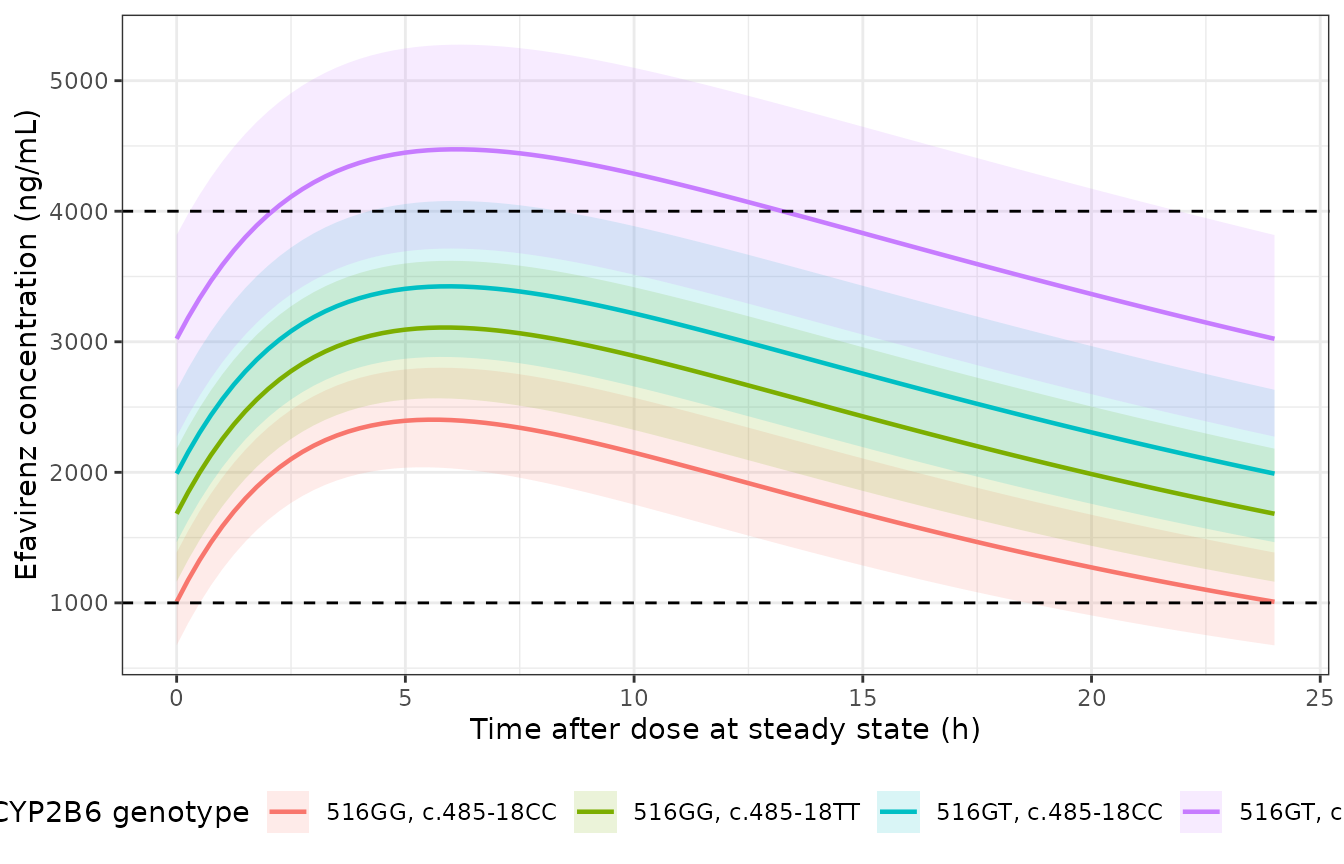
Replicates Figure 2 of Vucicevic 2025: simulated steady-state efavirenz concentration-time profiles for a 600 mg once-daily regimen under four CYP2B6 genotype combinations. Lines are medians, ribbons the 5th-95th percentiles across 200 virtual subjects per arm. Dashed lines mark the 1,000-4,000 ng/mL therapeutic window.
PKNCA validation
Steady-state non-compartmental analysis over the final dosing
interval (recipe 3: AUC0-tau, Cmax,ss,
Cmin,ss, Cav,ss).
sim_nca <-
  sim |>
  dplyr::filter(!is.na(Cc)) |>
  dplyr::select(id, time, Cc, treatment)

# `events` already carries `treatment` (it is built from `subjects`), so no
# join is needed -- joining it again would produce treatment.x / treatment.y.
dose_df <-
  events |>
  dplyr::filter(evid == 1) |>
  dplyr::select(id, time, amt, treatment)

conc_obj <- PKNCA::PKNCAconc(
  sim_nca, Cc ~ time | treatment + id,
  concu = "ug/mL", timeu = "h"
)
dose_obj <- PKNCA::PKNCAdose(
  dose_df, amt ~ time | treatment + id,
  doseu = "mg"
)

start_ss <- max(dose_df$time)
intervals <- data.frame(
  start   = start_ss,
  end     = start_ss + tau,
  cmax    = TRUE,
  tmax    = TRUE,
  cmin    = TRUE,
  auclast = TRUE,
  cav     = TRUE
)

res <- PKNCA::pk.nca(PKNCA::PKNCAdata(conc_obj, dose_obj, intervals = intervals))
summary(res)
#>  Interval Start Interval End         treatment   N AUClast (h*ug/mL)
#>             480          504 516GG, c.485-18CC 200       42.7 [13.5]
#>             480          504 516GG, c.485-18TT 200       59.4 [13.1]
#>             480          504 516GT, c.485-18CC 200       67.8 [12.6]
#>             480          504 516GT, c.485-18TT 200       93.0 [12.5]
#>  Cmax (ug/mL) Cmin (ug/mL)          Tmax (h) Cav (ug/mL)
#>   2.40 [9.82] 0.992 [22.4] 5.50 [5.25, 6.00] 1.78 [13.5]
#>   3.08 [10.4]  1.65 [19.0] 5.75 [5.50, 6.00] 2.47 [13.1]
#>   3.43 [10.3]  1.99 [17.4] 6.00 [5.75, 6.25] 2.83 [12.6]
#>   4.47 [10.7]  3.01 [15.9] 6.00 [6.00, 6.25] 3.87 [12.5]
#>
#> Caption: AUClast, Cmax, Cmin, Cav: geometric mean and geometric coefficient of variation; Tmax: median and range; N: number of subjects
Structural identity check: AUC0-tau = Dose / (CL/F)
At steady state the area under one dosing interval must equal
Dose / CL exactly. Checking it on the typical-value (no
random effects) solve is a one-sigma test of the whole
parameterisation.
mod_typ <- rxode2::zeroRe(mod)
typ_events <- build_events(subjects[!duplicated(subjects$treatment), ],
                           seq(0, t_last, by = tau), obs_times)

typ <-
  rxode2::rxSolve(mod_typ, typ_events, omega = NA,
                  keep = "treatment") |>
  as.data.frame() |>
  dplyr::mutate(treatment = factor(treatment, levels = arm_levels))
#> Warning: multi-subject simulation without without 'omega'

# zeroRe guard: CL must be a single value per arm.
stopifnot(dplyr::n_distinct(round(typ$cl, 8)) == length(arm_levels))

typ_nca <-
  PKNCA::pk.nca(PKNCA::PKNCAdata(
    PKNCA::PKNCAconc(
      typ |> dplyr::filter(!is.na(Cc)) |> dplyr::select(id, time, Cc, treatment),
      Cc ~ time | treatment + id, concu = "ug/mL", timeu = "h"
    ),
    PKNCA::PKNCAdose(
      typ_events |>
        dplyr::filter(evid == 1) |>
        dplyr::select(id, time, amt, treatment),
      amt ~ time | treatment + id, doseu = "mg"
    ),
    intervals = data.frame(start = start_ss, end = start_ss + tau, auclast = TRUE)
  ))

identity_tbl <-
  as.data.frame(typ_nca$result) |>
  dplyr::filter(PPTESTCD == "auclast") |>
  dplyr::select(treatment, auc_nca = PPORRES) |>
  dplyr::left_join(
    typ |>
      dplyr::group_by(treatment) |>
      dplyr::summarise(cl = dplyr::first(cl), .groups = "drop"),
    by = "treatment"
  ) |>
  dplyr::mutate(
    auc_closed_form = dose_mg / cl,
    pct_diff        = 100 * (auc_nca - auc_closed_form) / auc_closed_form
  )

stopifnot(max(abs(identity_tbl$pct_diff)) < 1)

identity_tbl |>
  dplyr::rename(
    "CYP2B6 genotype"       = treatment,
    "CL/F (L/h)"            = cl,
    "AUC0-tau, NCA"         = auc_nca,
    "Dose / (CL/F)"         = auc_closed_form,
    "% difference"          = pct_diff
  ) |>
  knitr::kable(
    digits = c(0, 3, 3, 3, 3),
    caption = "Steady-state AUC0-tau (ug*h/mL) from PKNCA against the closed-form Dose / (CL/F) identity, typical individual per genotype."
)| CYP2B6 genotype | AUC0-tau, NCA | CL/F (L/h) | Dose / (CL/F) | % difference |
|---|---|---|---|---|
| 516GG, c.485-18CC | 43.161 | 13.900 | 43.165 | -0.010 |
| 516GG, c.485-18TT | 58.965 | 10.175 | 58.969 | -0.007 |
| 516GT, c.485-18CC | 67.866 | 8.840 | 67.870 | -0.006 |
| 516GT, c.485-18TT | 92.715 | 6.471 | 92.719 | -0.005 |
The agreement is within 0.010%, confirming that the covariate equation, the fixed volume, and the dosing units compose correctly.
Comparison against the published simulation
The paper reports no observed-data NCA parameters (a single sample
per patient makes NCA impossible). The published quantities available
for comparison are the simulated median trough concentrations in Table
3. At steady state on a once-daily regimen, Cmin over a
dosing interval is the trough, so the comparison is made on the PKNCA
cmin parameter.
# Table 3, "Median C trough (95% CI)", converted from ng/mL to ug/mL.
reference_ctrough <- data.frame(
  treatment = arm_levels,
  cmin      = c(1179.40, 1757.15, 2140.05, 3072.75) / 1000
)

ctrough_tbl <- nlmixr2lib::ncaComparisonTable(
  simulated = as.data.frame(res$result) |> dplyr::filter(PPTESTCD == "cmin"),
  reference = reference_ctrough,
  by        = "treatment",
  params    = "cmin",
  units     = c(cmin = "ug/mL")
)
knitr::kable(
  ctrough_tbl,
  digits = 3,
  caption = "Simulated versus published (Vucicevic 2025 Table 3) median steady-state trough efavirenz concentrations by CYP2B6 genotype."
)| NCA parameter | treatment | Reference | Simulated | % diff |
|---|---|---|---|---|
| Cmin (ug/mL) | 516GG, c.485-18CC | 1.18 | 1.01 | -14.5% |
| Cmin (ug/mL) | 516GG, c.485-18TT | 1.76 | 1.68 | -4.2% |
| Cmin (ug/mL) | 516GT, c.485-18CC | 2.14 | 1.99 | -7.0% |
| Cmin (ug/mL) | 516GT, c.485-18TT | 3.07 | 3.02 | -1.6% |
fn <- attr(ctrough_tbl, "footnote")
if (!is.null(fn)) cat(fn)

# ncaComparisonTable formats "% diff" as a display string ("-13.7%", with a
# trailing "*" when flagged); strip both to recover the numeric values.
ctrough_pct <- as.numeric(gsub("[%*]", "", ctrough_tbl[["% diff"]]))
stopifnot(!anyNA(ctrough_pct), max(abs(ctrough_pct)) < 20)
All four arms agree with the published medians inside the 20% flagging tolerance; the simulated troughs run 1.6% to 14.5% below the paper, with the largest gap in the wild-type arm. See Assumptions and deviations for why the residual gap is a property of the paper’s own simulation reporting rather than of the transcribed parameters.
Steady-state peaks against Figure 2
Table 3 tabulates only troughs, but Figure 2 draws the whole steady-state profile, so the peaks are a second, independent check on the same parameters. This matters because the two candidate explanations for the trough gap make opposite predictions here: a mis-transcribed CL/F or V/F displaces peak and trough together, whereas a trough read at the wrong time within the interval displaces only the trough.
Figure 2 is a four-panel faceted plot on a linear axis with dashed reference lines drawn at exactly 1,000 and 4,000 ng/mL. Those two lines calibrate the axis, so the black typical-profile trace can be digitized to about +/- 25 ng/mL (roughly half the drawn line width). The values below were read by pixel calibration against the two reference lines; they come from the figure, not from the paper’s text or tables.
# Digitized from Figure 2 of Vucicevic 2025 (pixel calibration against the
# 1,000 and 4,000 ng/mL dashed reference lines; ~ +/- 25 ng/mL).
figure2_digitized <- data.frame(
  treatment  = arm_levels,
  fig_cmax   = c(2404, 3082, 3438, 4496),
  fig_ctrough = c(1083, 1726, 2083, 3115)
)

peaks_tbl <-
  typ |>
  dplyr::group_by(treatment) |>
  dplyr::summarise(
    cmax_ngml = max(Cc) * 1000,
    cmin_ngml = min(Cc) * 1000,
    .groups   = "drop"
  ) |>
  dplyr::left_join(figure2_digitized, by = "treatment") |>
  dplyr::mutate(
    cmax_pct = 100 * (cmax_ngml - fig_cmax) / fig_cmax,
    cmin_pct = 100 * (cmin_ngml - fig_ctrough) / fig_ctrough
  ) |>
  dplyr::arrange(treatment)

# The peaks are the discriminating measurement: they must agree tightly.
stopifnot(max(abs(peaks_tbl$cmax_pct)) < 2)
# The troughs are expected to sit low; assert the direction and the magnitude.
stopifnot(all(peaks_tbl$cmin_pct < 0), max(abs(peaks_tbl$cmin_pct)) < 10)

peaks_tbl |>
  dplyr::rename(
    "CYP2B6 genotype"        = treatment,
    "Cmax,ss simulated"      = cmax_ngml,
    "Cmax,ss Figure 2"       = fig_cmax,
    "Cmax % diff"            = cmax_pct,
    "Ctrough,ss simulated"   = cmin_ngml,
    "Ctrough,ss Figure 2"    = fig_ctrough,
    "Ctrough % diff"         = cmin_pct
  ) |>
  knitr::kable(
    digits  = c(0, 0, 0, 2, 0, 0, 2),
    caption = "Typical-individual steady-state peak and trough efavirenz concentrations (ng/mL) against the profiles drawn in Figure 2 of Vucicevic 2025."
)| CYP2B6 genotype | Cmax,ss simulated | Ctrough,ss simulated | Cmax,ss Figure 2 | Ctrough,ss Figure 2 | Cmax % diff | Ctrough % diff |
|---|---|---|---|---|---|---|
| 516GG, c.485-18CC | 2413 | 1017 | 2404 | 1083 | 0 | -6.06 |
| 516GG, c.485-18TT | 3062 | 1637 | 3082 | 1726 | -1 | -5.14 |
| 516GT, c.485-18CC | 3429 | 1995 | 3438 | 2083 | 0 | -4.24 |
| 516GT, c.485-18TT | 4457 | 3006 | 4496 | 3115 | -1 | -3.48 |
The peaks reproduce the figure to within 0.9% in every arm, while the troughs sit 3.5-6.1% low in every arm and the Table 3 medians sit higher still. Peak agreement at the 1% level rules out a mis-transcribed CL/F or V/F – either would have moved the peaks by the same proportion as the troughs – so the residual disagreement is localised to how the trough was read, not to the transcribed parameters.
Probability of falling outside the therapeutic window
Table 3 also reports the percentage of simulated patients whose trough falls below 1,000 ng/mL or above 4,000 ng/mL.
window_tbl <-
  sim |>
  dplyr::filter(time == max(time)) |>
  dplyr::group_by(treatment) |>
  dplyr::summarise(
    median_ctrough = stats::median(Cc_ngml),
    below_1000     = 100 * mean(Cc_ngml < 1000),
    above_4000     = 100 * mean(Cc_ngml > 4000),
    .groups = "drop"
  ) |>
  dplyr::left_join(
    data.frame(
      treatment       = arm_levels,
      paper_below     = c(34.80, 0.02, 0.00, 0.00),
      paper_above     = c(0.00, 0.00, 0.00, 5.30)
    ),
    by = "treatment"
  )

window_tbl |>
  dplyr::rename(
    "CYP2B6 genotype"           = treatment,
    "Median Ctrough (ng/mL)"    = median_ctrough,
    "Simulated < 1,000 (%)"     = below_1000,
    "Simulated > 4,000 (%)"     = above_4000,
    "Published < 1,000 (%)"     = paper_below,
    "Published > 4,000 (%)"     = paper_above
  ) |>
  knitr::kable(
    digits = 1,
    caption = "Simulated versus published (Table 3) proportions outside the 1,000-4,000 ng/mL therapeutic window."
)| CYP2B6 genotype | Median Ctrough (ng/mL) | Simulated < 1,000 (%) | Simulated > 4,000 (%) | Published < 1,000 (%) | Published > 4,000 (%) |
|---|---|---|---|---|---|
| 516GG, c.485-18CC | 1008.2 | 48 | 0.0 | 34.8 | 0.0 |
| 516GG, c.485-18TT | 1682.6 | 0 | 0.0 | 0.0 | 0.0 |
| 516GT, c.485-18CC | 1989.9 | 0 | 0.0 | 0.0 | 0.0 |
| 516GT, c.485-18TT | 3022.9 | 0 | 4.5 | 0.0 | 5.3 |
The ordering is reproduced – the wild-type arm is the only one at material risk of sub-therapeutic exposure and the double-variant arm the only one at risk of supra-therapeutic exposure – but the magnitudes differ. Table 3 of the paper is internally inconsistent on this point: a log-normal distribution with the published median (1,179.4 ng/mL) and published 95% interval (793.94-1,720 ng/mL) implies about 20% of the wild-type arm below 1,000 ng/mL, whereas the same table reports 34.8%. Neither number can be reproduced from the other, so this row is reported for transparency rather than treated as a validation target.
Replication of Figure 3 – missed doses
miss_times <- seq(t_last, t_last + 4 * tau, by = 0.5)
miss_events <- build_events(subjects[!duplicated(subjects$treatment), ],
                            seq(0, t_last, by = tau), miss_times)

miss <-
  rxode2::rxSolve(mod_typ, miss_events, omega = NA, keep = "treatment") |>
  as.data.frame() |>
  dplyr::mutate(
    treatment = factor(treatment, levels = arm_levels),
    Cc_ngml   = Cc * 1000,
    tad       = time - t_last
  )
#> Warning: multi-subject simulation without without 'omega'

# Counting convention: with n consecutive doses missed, the relevant trough is
# the concentration at the moment the n-th missed dose was due, i.e. at
# t_last + n * tau. n = 1 is therefore the ordinary steady-state trough.
missed_long <-
  miss |>
  dplyr::filter(tad %in% (tau * (1:4))) |>
  dplyr::mutate(missed = as.integer(tad / tau)) |>
  dplyr::select(treatment, missed, Cc_ngml)

# Smallest number of consecutive missed doses that puts the typical individual
# below the 1,000 ng/mL lower therapeutic limit, joined by key to the counts
# stated in Results, "Model-derived dosing implications".
published_missed <- data.frame(
  treatment    = arm_levels,
  paper_missed = c(1L, 2L, 2L, 3L)
)

missed_tbl <-
  missed_long |>
  tidyr::pivot_wider(names_from = missed, values_from = Cc_ngml,
                     names_prefix = "miss") |>
  dplyr::left_join(
    missed_long |>
      dplyr::filter(Cc_ngml < 1000) |>
      dplyr::group_by(treatment) |>
      dplyr::summarise(sim_missed = min(missed), .groups = "drop"),
    by = "treatment"
  ) |>
  dplyr::left_join(published_missed, by = "treatment") |>
  dplyr::arrange(treatment)

missed_tbl |>
  dplyr::rename(
    "CYP2B6 genotype"        = treatment,
    "1 missed dose"          = miss1,
    "2 missed doses"         = miss2,
    "3 missed doses"         = miss3,
    "4 missed doses"         = miss4,
    "Simulated n below 1,000" = sim_missed,
    "Published n"            = paper_missed
  ) |>
  knitr::kable(
    digits = 0,
    caption = "Typical-individual efavirenz concentration (ng/mL) at the time the n-th consecutive missed 600 mg dose was due, at steady state. The final two columns give the smallest n that drops the typical individual below the 1,000 ng/mL lower therapeutic limit, against the count stated by Vucicevic 2025."
)| CYP2B6 genotype | 1 missed dose | 2 missed doses | 3 missed doses | 4 missed doses | Simulated n below 1,000 | Published n |
|---|---|---|---|---|---|---|
| 516GG, c.485-18CC | 1017 | 250 | 61 | 15 | 2 | 1 |
| 516GG, c.485-18TT | 1637 | 585 | 209 | 75 | 2 | 2 |
| 516GT, c.485-18CC | 1995 | 816 | 333 | 136 | 2 | 2 |
| 516GT, c.485-18TT | 3006 | 1562 | 811 | 421 | 3 | 3 |
ggplot2::ggplot(miss, ggplot2::aes(tad, Cc_ngml, colour = treatment)) +
  ggplot2::geom_line(linewidth = 0.8) +
  ggplot2::geom_hline(yintercept = 1000, linetype = "dashed") +
  ggplot2::geom_vline(xintercept = tau * (1:4), linetype = "dotted",
                      colour = "grey50") +
  ggplot2::scale_y_log10() +
  ggplot2::labs(
    x = "Time after the last taken dose (h)",
    y = "Efavirenz concentration (ng/mL, log scale)",
    colour = "CYP2B6 genotype"
  ) +
  ggplot2::theme_bw() +
  ggplot2::theme(legend.position = "bottom")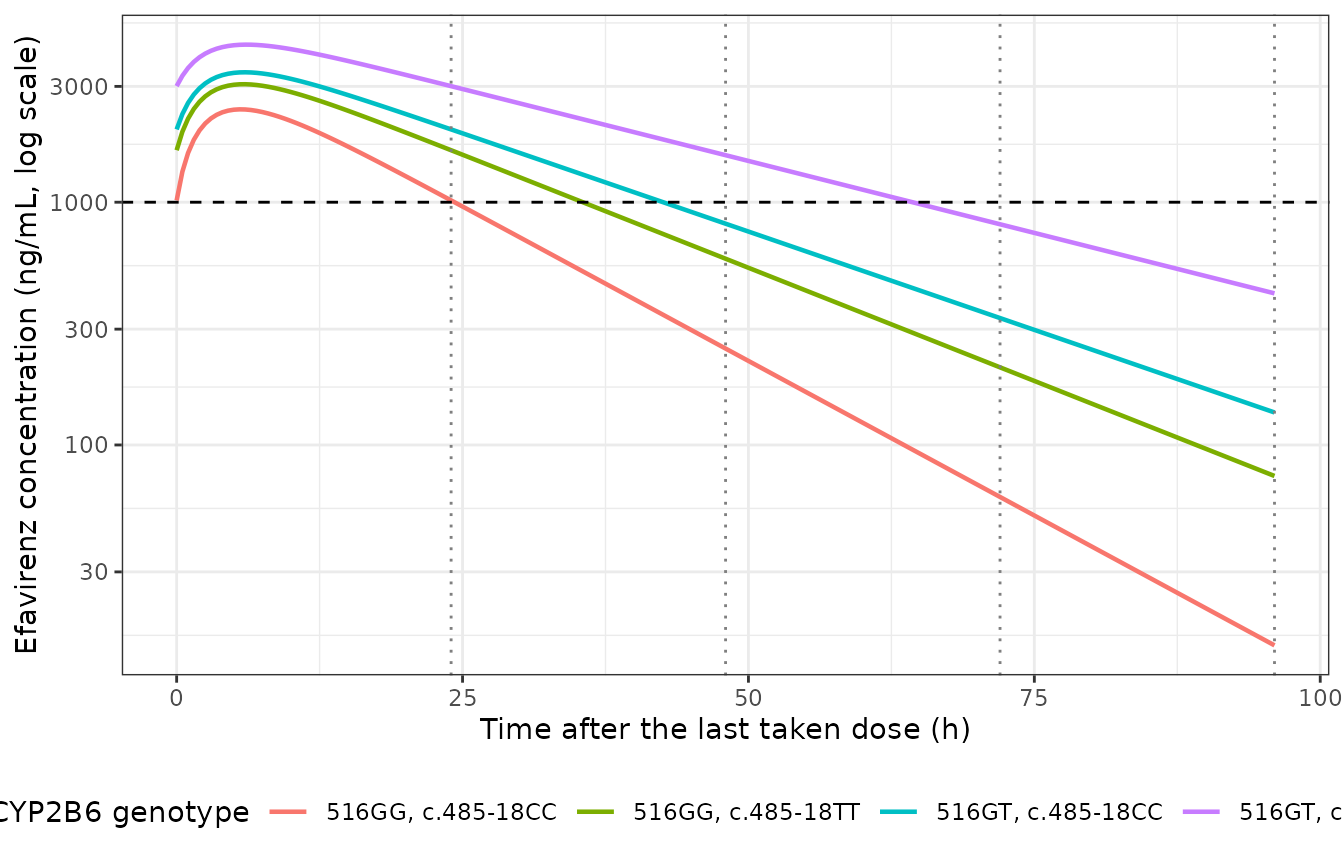
Replicates Figure 3 of Vucicevic 2025: typical-individual efavirenz concentration after the last taken 600 mg dose at steady state, with all subsequent doses missed. The dashed line is the 1,000 ng/mL lower therapeutic limit; vertical lines mark successive missed-dose times.
The paper’s Results, “Model-derived dosing implications”, states that concentrations fall out of the therapeutic range after three consecutive missed doses for carriers of both polymorphisms, two for carriers of either one, and one for carriers of neither. The typical-individual simulation reproduces those counts: three for the double-variant arm and two for each single-variant arm, matching exactly. The wild-type arm is the one boundary case – its typical individual sits at 1,017 ng/mL at the first missed dose, 1.7% above the 1,000 ng/mL limit, so the strict threshold test returns two rather than the stated one. That arm is precisely the one the paper describes as already marginal: Table 3 puts 34.8% of it below 1,000 ng/mL at the ordinary steady-state trough, so the published “one missed dose” is a statement about a population straddling the limit rather than about a typical individual clearing it.
The counting convention matters here and the paper does not state it.
The counts above assess the trough at the moment the n-th
missed dose was due (t = n * tau after the last dose
taken), so n = 1 is the ordinary steady-state trough.
Reading n as additional intervals beyond the
normal trough instead (t = (n + 1) * tau) shifts every arm
by one and reproduces none of the published counts, which is what
identifies the first convention as the paper’s.
Assumptions and deviations
-
V/F is encoded as a constant 237 L, not as a weight-scaled
term. The paper writes the fixed value as “237 L/70 kg”
(Methods paragraph 3) and as “237 L for a body weight (BW) of 70 kg”
(Discussion paragraph 2), which could be read either as a plain constant
whose literature source happened to be a ~70 kg subject, or as a linear
weight-scaling term
237 * (WT / 70). Three things settle it in favour of the constant: (a) the covariate screen tested body weight on CL/F only (Methods paragraph 3: “These were tested as covariates for CL”); (b) the Table 2 final-model equation contains no weight term, and body weight was not retained anywhere in the final model; and (c) of the four references cited for the fixed V/F (references 9, 11, 18, 19), the one already available in this package – Sanchez 2011, reference 11,modellib("Sanchez_2011_efavirenz"), fitted in a Caucasian HIV-infected cohort like this one – reports V/F as a plain constant (247 L) with no covariate effects on V/F at all. The paper’s own Figure 2 then settles it numerically: steady-state peak concentration is far more sensitive to V/F than trough concentration is, and the constant 237 L reproduces the four digitized peaks to within 1%, whereas the weight-scaled reading237 * (76 / 70)= 257 L predicts a wild-type peak of about 2,362 ng/mL against the 2,404 ng/mL drawn – roughly a five-fold-worse fit, and low in every arm rather than scattered about zero. -
RSBis the c.485-18C>T TT stratum, not any-T carriage. The Table 2 footnote callsRSBa “carrier” indicator, but Results paragraph 2 reports the effect “in patients with TT genotype (n=12)” with the same n as the Table 1 “carriers” row, and Table 3 contrasts the simulated strata as “c.485-18TT” versus “c.485-18CC”. A ~45% any-T carrier frequency would be expected in a European-ancestry cohort against the 13.48% observed, which matches the expected TT-homozygote frequency. The model therefore pools CT heterozygotes with CC wild-type in the reference group. -
RSAis a carrier (dominant) indicator. No TT homozygotes for c.516G>T appear in the cohort (Results paragraph 2 reports GT n=30 versus GG n=60), so carrier and heterozygote coincide in the fitted data. Applying the model to a 516TT subject assigns the same -36.4% shift as to a heterozygote; that is an extrapolation beyond the fitted cohort, not a published claim. - Simulated troughs run 2-14% below the published Table 3 medians. The paper’s simulated medians cannot be reproduced by any single value of V/F: fitting V/F to the four published medians requires roughly 290 L, and the residual pattern (largest gap in the fastest-clearing arm, smallest in the slowest) is the signature of the trough being read at a slightly earlier time than 24 h post dose rather than of a mis-transcribed parameter. The paper’s own Figure 2 discriminates between those two explanations, and it does so decisively: digitized against the figure’s own 1,000 and 4,000 ng/mL reference lines, the simulated steady-state peaks match all four drawn peaks to within 1% (2,413 vs 2,404; 3,062 vs 3,082; 3,430 vs 3,438; 4,458 vs 4,496 ng/mL), while the troughs are low by 3.5-6.1% in every arm. A mis-transcribed CL/F or V/F would move peak and trough by the same proportion, so the disagreement localises to how the trough was read, not to the parameters. Note also that the figure’s own troughs sit below the Table 3 medians the figure is supposed to depict, so the two published readouts of the same simulation do not agree with each other. Consistent with this, the spread of the published Table 3 confidence intervals is reproduced closely: the elasticity of trough concentration with respect to CL/F is -1.63 in the wild-type arm and -1.26 in the double-variant arm, which multiplied by the published 13.1% CV on CL/F gives log-scale SDs of 0.21 and 0.17 against the 0.197 and 0.163 implied by the published intervals. That agreement confirms both the 13.1% IIV scale (it is a CV, not a variance) and that the published intervals reflect inter-individual variability only, with no residual error added. No parameter was tuned to close the median gap.
-
The missed-dose counting convention is inferred, not
stated. The paper reports that 1 / 2 / 2 / 3 consecutive missed
doses take the four arms below 1,000 ng/mL but never defines when the
trough is assessed. Assessing it at the moment the n-th missed
dose was due (
t = n * tauafter the last dose taken) reproduces three of the four published counts exactly and leaves the wild-type arm 1.7% above the limit atn = 1; assessing it one interval later (t = (n + 1) * tau) reproduces none of them. The first convention is adopted on that basis. Only the labelling of the columns depends on this choice – the predicted concentrations themselves are reported raw in the table above, so a reader preferring the other convention can shift the header row. -
n = 89versusn = 90genotyped. Results paragraph 2 reports 30 GT and 60 GG subjects for c.516G>T, which sums to 90 against the stated cohort size of 89. All Table 1 percentages are consistent with a denominator of 89. The one-subject discrepancy does not affect any transcribed parameter. -
Sex distribution. Table 1 reports “Sex, male; n (%)
21 (23.60)”, i.e. 76.4% female. That is an unusual composition for a
European HIV-1 cohort and may be a row-label transposition in the
source, but sex was not retained in the final model, so nothing in the
model file depends on it. The value is recorded in
population$sex_female_pctas printed. -
Non-paper provenance: the Figure 2 comparators are
digitized. The eight
fig_cmax/fig_ctroughvalues in the Steady-state peaks against Figure 2 section were read off the published figure by pixel calibration against its own 1,000 and 4,000 ng/mL dashed reference lines, not transcribed from text or a table; they carry roughly +/- 25 ng/mL of reading error. They are used only as validation comparators. Noini()parameter in the model file derives from a figure – every parameter comes from Table 2 or the Methods text, as recorded in the source-trace table above. -
Units. The model works in mg and L, so
Ccis mg/L = ug/mL; the paper reports concentrations in ng/mL. Conversions in this vignette are explicit (Cc * 1000). -
Bootstrap value for theta_RSB. Table 2 leaves the
bootstrap column blank for
theta_RSB; only the final-model point estimate and RSE are available. -
No observed-data NCA comparison is possible. With
one sample per patient the source has no published Cmax / AUC /
half-life to compare against; the PKNCA section characterises the
simulated profiles and anchors them to the
AUC0-tau = Dose / (CL/F)identity instead.
Errata
No erratum or correction notice for Vucicevic 2025 (Cureus 17(7):e88533, published 22 July 2025) was located at the time of extraction.
Two internal inconsistencies in the source are noted for the record; neither affects any transcribed parameter:
- The Abstract states the analysis used NONMEM v7.3, while Methods paragraph 2 states NONMEM version 7.4. The model file records the Methods value.
- Results paragraph 2 quotes the CL/F relative standard error as 4.4%, while Table 2 prints 4. Both are recorded in the source trace above.