Co-trimoxazole: sulfamethoxazole and trimethoprim (Chen 2025)
Source:vignettes/articles/Chen_2025_cotrimoxazole.Rmd
Chen_2025_cotrimoxazole.RmdModel and source
Chen 2025 fitted two independent one-compartment models, one per component of the fixed-dose combination, so the paper contributes two model files and this single vignette.
#> ℹ parameter labels from comments will be replaced by 'label()'
#> ℹ parameter labels from comments will be replaced by 'label()'- Citation: Chen B, Chen Y, Chen M, Mao Y, Huang Y, Zhou L, Wu W, Li X, Wu X, Cheng Y, Qiu H. Population pharmacokinetics and Monte Carlo-based dosing optimization of trimethoprim-sulfamethoxazole. Antimicrob Agents Chemother. 2025;69(11):e00519-25. doi:10.1128/aac.00519-25. Structural equations from Eq. 1 and Eq. 2 of the Results section (‘Population pharmacokinetic analysis’); fixed effects, interindividual variability and residual error from Table 5. The equations are rendered as images in the publisher PDF and were recovered with ‘pdftotext -layout’.
- Article: https://doi.org/10.1128/aac.00519-25 (PMC12587597, open access)
Sulfamethoxazole – One-compartment population PK model for INTRAVENOUS sulfamethoxazole in adults treated with co-trimoxazole for Pneumocystis jirovecii pneumonia (Chen 2025). Both the typical volume and the typical clearance are reported per kilogram of body weight (L/kg and L/kg/h), so body weight enters both parameters linearly; this is how the ‘WT on CL’ step retained in the covariate search is carried, and it is why the printed model equations show no explicit weight term. Creatinine clearance scales clearance as a power function normalized to the cohort median of 75.7 mL/min, and continuous renal replacement therapy multiplies clearance by exp(0.59) = 1.80 because sulfamethoxazole is removed by ultrafiltration and is not reabsorbed in the ultrafiltrate. Doses are the SULFAMETHOXAZOLE component of the combination product: a co-trimoxazole dose of X mg/kg/day delivers 5X/6 mg/kg/day of sulfamethoxazole and X/6 mg/kg/day of trimethoprim. The trimethoprim model of the same paper is a separate file; see modellib(‘Chen_2025_trimethoprim’).
Trimethoprim – One-compartment population PK model for INTRAVENOUS trimethoprim in adults treated with co-trimoxazole for Pneumocystis jirovecii pneumonia (Chen 2025). Both the typical volume and the typical clearance are reported per kilogram of body weight (L/kg and L/kg/h), so body weight enters both parameters linearly; this is how the ‘WT on CL’ step retained in the covariate search is carried, and it is why the printed model equations show no explicit weight term. Creatinine clearance scales clearance as a power function normalized to the cohort median of 75.7 mL/min. Unlike the companion sulfamethoxazole model, continuous renal replacement therapy is NOT a covariate here: trimethoprim has a large volume of distribution and is about 60% protein bound, so little is removed by ultrafiltration. NOTE the typical volume is taken as 2.22 L/kg from the Discussion rather than the 8.22 L/kg printed in Table 6; four independent lines of evidence refute 8.22 and the vignette Errata sets them out in full. Doses are the TRIMETHOPRIM component of the combination product: a co-trimoxazole dose of X mg/kg/day delivers X/6 mg/kg/day of trimethoprim and 5X/6 mg/kg/day of sulfamethoxazole. The sulfamethoxazole model of the same paper is a separate file; see modellib(‘Chen_2025_sulfamethoxazole’).
The publisher PDF renders the four model equations as images, so they
do not survive plain-text extraction of the PDF. They were recovered
with pdftotext -layout:
(1)  V  = tvV * exp(etaV)                                                    [SMX]
(2)  CL = tvCL * (CrCL/75.7)^dCLdCrCL * exp[dCLdCRRT * (CRRT == 1)] * exp(etaCL)
(3)  V  = tvV * exp(etaV)                                                    [TMP]
(4)  CL = tvCL * (CrCL/75.7)^dCLdCrCL * exp(etaCL)
Neither equation carries a weight term, because Tables 5 and 6 report
tvV in L/kg and tvCL in
L/kg/h. Body weight therefore enters both parameters
linearly, and that per-kg parameterisation is how the “WT on CL” step
retained by the forward/backward search (Table 3 model 7, Table 4 model
6) is carried. model() makes it explicit as
vc <- exp(lvc + etalvc) * WT.
Population
79 adults with confirmed Pneumocystis jirovecii pneumonia, treated with intravenous co-trimoxazole at Fujian Medical University Union Hospital between March 2023 and October 2024, in intensive care units and general wards (Table 2). The cohort was 77.2% male, median age 64 years (54-73), median height 170 cm (165-175) and median weight 60.0 kg (55-70). Renal function was frequently impaired: median Cockcroft-Gault creatinine clearance 75.7 mL/min (51.0-93.7), with 47 of 79 patients (59.5%) below 80 mL/min and 19 (24.1%) receiving continuous renal replacement therapy. Hepatic function spanned Child-Pugh A (54), B (18) and C (7). NAT2 acetylator phenotype and CYP2C9 metabolizer phenotype were genotyped; neither, nor any liver-function marker, reached significance.
232 post-dose plasma concentrations were available, two to three per patient (an end-of-infusion peak, a pre-dose trough and/or an intermediate sample; Table 1), assayed by LC-MS/MS over 3.12-400.0 mg/L for sulfamethoxazole and 0.20-25.0 mg/L for trimethoprim. Infusions lasted approximately 1 h and were given every 6, 8 or 12 h. Estimation used first-order conditional estimation with extended least squares in Phoenix NLME 8.0.
The same information is available programmatically via
readModelDb("Chen_2025_sulfamethoxazole")()$population.
Source trace
| Equation / parameter | Value | Source location |
|---|---|---|
| Sulfamethoxazole | ||
d/dt(central), one compartment, first-order
elimination |
n/a | Results, “Population pharmacokinetic analysis”; Table 3 model 1 (OFV 2,091.68) beats model 2, two compartments (2,123.61) |
V = tvV * exp(etaV) |
n/a | Equation 1 |
CL = tvCL * (CrCL/75.7)^dCLdCrCL * exp[dCLdCRRT*(CRRT==1)] * exp(etaCL) |
n/a | Equation 2 |
lvc (tv V) |
0.32 L/kg | Table 5; Discussion confirms “0.32 L/kg for SMX” |
lcl (tv CL) |
0.02 L/kg/h | Table 5; Discussion confirms “0.02 L/kg/h for SMX” |
e_crcl_cl (dCLdCrCL) |
0.17 | Table 5 |
e_rrt_crrt_status_cl (dCLdCRRT) |
0.59 (log scale; 1.80-fold) | Table 5, entering inside exp() per Equation 2 |
etalvc |
0.08 (variance) | Table 5 “omega^2 V”; footnote: “omega^2, variance of interindividual variability” |
etalcl |
0.16 (variance) | Table 5 “omega^2 CL” |
propSd |
0.09 | Table 5 “Proportional error”; Table 3 selects the proportional model on OFV |
| normalising CrCL | 75.7 mL/min | Sentence after Equations 1-4: “75.7 represents the median CrCL value”; Table 2 median |
| Trimethoprim | ||
d/dt(central), one compartment, first-order
elimination |
n/a | Results; Table 4 model 1 (OFV 559.47) beats model 2 (579.49) |
V = tvV * exp(etaV) |
n/a | Equation 3 |
CL = tvCL * (CrCL/75.7)^dCLdCrCL * exp(etaCL) |
n/a | Equation 4 (no CRRT term) |
lvc (tv V) |
2.22 L/kg | Discussion, not Table 6 – see Errata below |
lcl (tv CL) |
0.11 L/kg/h | Table 6; Discussion confirms “0.11 L/kg/h for TMP” |
e_crcl_cl (dCLdCrCL) |
0.29 | Table 6 |
etalvc |
0.19 (variance) | Table 6 “omega^2 V” |
etalcl |
0.25 (variance) | Table 6 “omega^2 CL” |
propSd |
0.27 | Table 6 “Proportional error”, “Final model / Estimate” column |
| Both | ||
| Efficacy / toxicity window | SMX 100-200 mg/L, TMP 5-10 mg/L | Methods, “Monte Carlo simulation”; Table 7 column headers |
| Dose ladder by renal function | see Table 7 | Table 7 |
Published parameter values, transcribed once
Every published number the validation uses is typed literally here,
so the checks below compare the packaged model against the
paper, not against itself. A mis-transcription in
either .R file turns these gates red.
pub <- list(
  smx = list(v = 0.32, cl = 0.02, e_crcl = 0.17, e_crrt = 0.59,
             lo = 100, hi = 200),
  tmp = list(v = 2.22, cl = 0.11, e_crcl = 0.29, e_crrt = 0,
             lo = 5,   hi = 10)
)
ref_crcl <- 75.7   # median CrCL, stated after Equations 1-4
tinf     <- 1      # "each infusion time lasting approximately 1 h" (Methods)
wt_med   <- 60     # cohort median weight, Table 2

# Co-trimoxazole is dosed as a whole; the paper states 90-120 mg/kg/day is
# "equivalent to SMX 75-100 mg/kg/day and TMP 15-20 mg/kg/day", i.e. a 5:1
# split, so SMX takes 5/6 of the total and TMP 1/6.
frac <- c(smx = 5 / 6, tmp = 1 / 6)

# Table 7: recommended regimen per renal-function stratum. `crcl` is the
# midpoint of each printed band. The paper does not report the CRRT subgroup's
# own creatinine clearance, so the cohort median is used there and the arm is
# flagged; Table 7 leaves the CRRT row's TMP cells blank because the model
# found no CRRT effect on trimethoprim.
arms_t7 <- tibble::tribble(
  ~treatment,       ~crcl, ~crrt, ~daily, ~nday, ~tmp_ok,
  "CrCL <15",         10,      0,     50,     3,    TRUE,
  "CrCL 15-29",       22,      0,     55,     3,    TRUE,
  "CrCL 30-49",       40,      0,     55,     2,    TRUE,
  "CrCL 50-79",       65,      0,     65,     3,    TRUE,
  "CrCL 80-120",     100,      0,     70,     3,    TRUE,
  "CRRT",           75.7,      1,     90,     3,   FALSE
)

# Discussion: at 90 mg/kg/day and normal renal function the fraction of patients
# above the toxicity threshold rises as the same daily dose is split into fewer
# infusions (SMX 35% q6h vs 67.3% q12h; TMP 20% q6h vs 45.8% q12h).
arms_freq <- tibble::tribble(
  ~treatment,        ~crcl, ~crrt, ~daily, ~nday, ~tmp_ok,
  "90 mg/kg/day QID",  100,     0,     90,     4,    TRUE,
  "90 mg/kg/day TID",  100,     0,     90,     3,    TRUE,
  "90 mg/kg/day BID",  100,     0,     90,     2,    TRUE
)

arms <- dplyr::bind_rows(arms_t7, arms_freq) |>
  dplyr::mutate(tau = 24 / nday)
Closed-form reference
For a one-compartment model given a tinf-hour infusion
every tau hours, the steady-state peak, trough, average and
interval AUC have exact expressions. These are computed
only from the published constants above – no model
object is touched – so they are an independent reference for the
solver.
# Typical (no-eta) clearance and volume in absolute units, from published values
pub_cl <- function(d, crcl, crrt, wt = wt_med) {
  p <- pub[[d]]
  p$cl * wt * (crcl / ref_crcl)^p$e_crcl * exp(p$e_crrt * crrt)
}
pub_vc <- function(d, wt = wt_med) pub[[d]]$v * wt

# Steady-state metrics for a constant-rate infusion repeated every tau hours.
ss_metrics <- function(dose, tau, cl, vc, tinf. = tinf) {
  k    <- cl / vc
  rate <- dose / tinf.
  cmax <- (rate / cl) * (1 - exp(-k * tinf.)) / (1 - exp(-k * tau))
  cmin <- cmax * exp(-k * (tau - tinf.))
  list(cmax = cmax, cmin = cmin,
       cav = dose / (cl * tau), auclast = dose / cl,
       half.life = log(2) / k)
}

closed <- arms |>
  tidyr::expand_grid(drug = c("smx", "tmp")) |>
  dplyr::filter(drug == "smx" | tmp_ok) |>
  dplyr::mutate(
    dose = daily * frac[drug] / nday * wt_med,
    cl   = mapply(pub_cl, drug, crcl, crrt),
    vc   = vapply(drug, pub_vc, numeric(1))
  ) |>
  dplyr::rowwise() |>
  dplyr::mutate(m = list(ss_metrics(dose, tau, cl, vc))) |>
  dplyr::ungroup() |>
  tidyr::unnest_wider(m)

closed |>
  dplyr::filter(treatment %in% arms_t7$treatment) |>
  dplyr::transmute(
    Drug = toupper(drug), Stratum = treatment,
    `Regimen (mg/kg/day)` = sprintf("%s %g", c("BID", "TID", "QID")[nday - 1], daily),
    `CL (L/h)` = round(cl, 3), `t1/2 (h)` = round(half.life, 1),
    `Cmax,ss (mg/L)` = round(cmax, 1), `Cmin,ss (mg/L)` = round(cmin, 1)
  ) |>
knitr::kable(caption = "Closed-form steady-state metrics from the PUBLISHED parameter values at the Table 7 recommended regimens (60 kg).")| Drug | Stratum | Regimen (mg/kg/day) | CL (L/h) | t1/2 (h) | Cmax,ss (mg/L) | Cmin,ss (mg/L) |
|---|---|---|---|---|---|---|
| SMX | CrCL <15 | TID 50 | 0.851 | 15.6 | 142.3 | 104.3 |
| TMP | CrCL <15 | TID 50 | 3.669 | 25.2 | 6.2 | 5.1 |
| SMX | CrCL 15-29 | TID 55 | 0.973 | 13.7 | 139.7 | 98.0 |
| TMP | CrCL 15-29 | TID 55 | 4.612 | 20.0 | 5.6 | 4.4 |
| SMX | CrCL 30-49 | BID 55 | 1.077 | 12.4 | 142.2 | 76.7 |
| TMP | CrCL 30-49 | BID 55 | 5.485 | 16.8 | 5.2 | 3.3 |
| SMX | CrCL 50-79 | TID 65 | 1.169 | 11.4 | 141.9 | 92.7 |
| TMP | CrCL 50-79 | TID 65 | 6.315 | 14.6 | 5.0 | 3.6 |
| SMX | CrCL 80-120 | TID 70 | 1.258 | 10.6 | 144.2 | 91.1 |
| TMP | CrCL 80-120 | TID 70 | 7.155 | 12.9 | 4.9 | 3.4 |
| SMX | CRRT | TID 90 | 2.165 | 6.1 | 124.3 | 56.5 |
Virtual cohort and simulation
Original observed data are not public. Because both V
and CL are per-kg and every recommended dose is in mg/kg,
simulated concentrations do not depend on the weight supplied – the
cohort median 60 kg is used throughout. Creatinine clearance is drawn
uniformly inside each published band, mirroring the paper’s own
stratification.
Dosing runs for 15 days so that every arm is at steady state (the
longest half-life in the ladder is about 25 h, in the trimethoprim
CrCL <15 arm, so 15 days is more than 14 half-lives).
Observations are placed over the final dosing interval.
# set.seed() seeds R's RNG only. rxode2's simulation streams are partitioned per
# solver thread, so this cohort is NOT reproducible across machines with
# different thread counts; every assertion below is written to hold for any
# cohort the model can produce.
set.seed(20250903)

horizon    <- 15 * 24
n_per_arm  <- 100          # within the 200-per-arm cohort cap

# One arm's event table. `id_offset` keeps IDs disjoint across arms; duplicate
# IDs are silently merged by rxSolve into a single over-dosed subject.
make_arm <- function(arm, drug, n, id_offset, fine = 0.1, coarse = NA) {
  dose_amt  <- arm$daily * frac[[drug]] / arm$nday * wt_med
  dose_time <- seq(0, horizon - arm$tau, by = arm$tau)
  t_last    <- max(dose_time)

  subj <- tibble::tibble(
    id   = id_offset + seq_len(n),
    WT   = wt_med,
    CRCL = if (n == 1) arm$crcl else stats::runif(n, arm$crcl_lo, arm$crcl_hi),
    RRT_CRRT_STATUS = arm$crrt,
    treatment = arm$treatment
  )

  obs_t <- seq(t_last, horizon, by = fine)
  if (!is.na(coarse)) obs_t <- sort(unique(c(seq(0, horizon, by = coarse), obs_t)))

  dplyr::bind_rows(
    tidyr::expand_grid(subj, time = dose_time) |>
      dplyr::mutate(amt = dose_amt, evid = 1L, cmt = "central",
                    rate = dose_amt / tinf),
    tidyr::expand_grid(subj, time = obs_t) |>
      dplyr::mutate(amt = NA_real_, evid = 0L, cmt = "central",
                    rate = 0)
  ) |>
    dplyr::arrange(id, time, dplyr::desc(evid))
}

# Uniform CrCL band per arm for the stochastic cohort.
arms <- arms |>
  dplyr::mutate(
    crcl_lo = c(5, 15, 30, 50, 80, 75.7, 80, 80, 80),
    crcl_hi = c(15, 29, 49, 79, 120, 75.7, 120, 120, 120)
  )

build_events <- function(drug, n, fine, coarse = NA) {
  keep <- if (drug == "tmp") dplyr::filter(arms, tmp_ok) else arms
  out  <- vector("list", nrow(keep))
  for (i in seq_len(nrow(keep))) {
    out[[i]] <- make_arm(keep[i, ], drug, n, id_offset = (i - 1L) * 1000L,
                         fine = fine, coarse = coarse)
  }
  dplyr::bind_rows(out)
}

# Typical-value events: one deterministic subject per arm, plus a coarse grid
# from time 0 so the profile figure has a run-in.
ev_typ <- lapply(c(smx = "smx", tmp = "tmp"), build_events,
                 n = 1, fine = 0.05, coarse = 2)
# Stochastic events for the target-attainment reproduction.
ev_iiv <- lapply(c(smx = "smx", tmp = "tmp"), build_events,
                 n = n_per_arm, fine = 0.1)

for (e in c(ev_typ, ev_iiv)) {
  stopifnot(!anyDuplicated(unique(e[, c("id", "time", "evid")])))
}
mod <- list(smx = readModelDb("Chen_2025_sulfamethoxazole"),
            tmp = readModelDb("Chen_2025_trimethoprim"))

sim_typ <- lapply(names(mod), function(d) {
  rxode2::rxSolve(rxode2::zeroRe(mod[[d]]), events = as.data.frame(ev_typ[[d]]),
                  keep = "treatment") |>
    as.data.frame() |>
    dplyr::mutate(drug = d, treatment = as.character(treatment))
})
#> ℹ parameter labels from comments will be replaced by 'label()'
#> ℹ omega/sigma items treated as zero: 'etalvc', 'etalcl'
#> Warning: multi-subject simulation without without 'omega'
#> ℹ parameter labels from comments will be replaced by 'label()'
#> ℹ omega/sigma items treated as zero: 'etalvc', 'etalcl'
#> Warning: multi-subject simulation without without 'omega'
names(sim_typ) <- names(mod)

sim_iiv <- lapply(names(mod), function(d) {
  rxode2::rxSolve(mod[[d]], events = as.data.frame(ev_iiv[[d]]),
                  keep = "treatment") |>
    as.data.frame() |>
    dplyr::mutate(drug = d, treatment = as.character(treatment))
})
#> ℹ parameter labels from comments will be replaced by 'label()'
#> ℹ parameter labels from comments will be replaced by 'label()'
names(sim_iiv) <- names(mod)

stopifnot(
  all(vapply(sim_typ, function(s) all(is.finite(s$Cc)) && all(s$Cc >= 0), logical(1))),
  all(vapply(sim_iiv, function(s) all(is.finite(s$Cc)) && all(s$Cc >= 0), logical(1)))
)
Steady-state profiles at the recommended regimens
t_start <- horizon - max(arms$tau)

dplyr::bind_rows(sim_typ) |>
  dplyr::filter(treatment %in% arms_t7$treatment, time >= horizon - 24) |>
  dplyr::mutate(
    drug = factor(drug, c("smx", "tmp"),
                  c("Sulfamethoxazole", "Trimethoprim")),
    treatment = factor(treatment, arms_t7$treatment),
    time = time - (horizon - 24)
  ) |>
  ggplot(aes(time, Cc, colour = treatment)) +
  geom_line(linewidth = 0.7) +
  facet_wrap(~drug, scales = "free_y") +
  geom_hline(data = data.frame(
    drug = factor(rep(c("Sulfamethoxazole", "Trimethoprim"), each = 2)),
    y    = c(100, 200, 5, 10)),
    aes(yintercept = y), inherit.aes = FALSE,
    linetype = "dashed", colour = "grey40") +
  labs(x = "Time within the final 24 h (h)", y = "Concentration (mg/L)",
       colour = "Renal stratum",
       title = "Typical-value steady-state profiles at the Table 7 doses",
       caption = paste("Dashed lines are the efficacy / toxicity window",
                       "(SMX 100-200, TMP 5-10 mg/L). Companion to Figures 4 and 5",
                       "of Chen 2025."))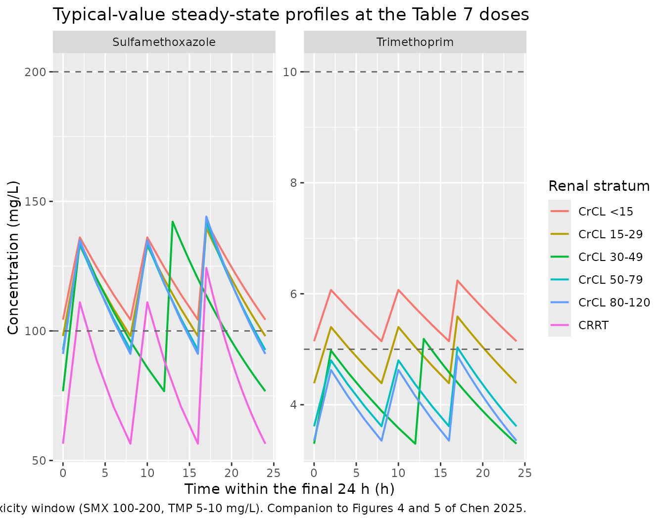
Validation
Solver against the closed form
The rxode2 solution over the final dosing interval is compared with the analytic steady-state expressions built from the published constants. This is a deterministic comparison of two independent computations, so the tolerance is tight; a mis-transcribed volume, clearance or exponent moves it by tens of percent.
last_interval <- function(s, arm_tbl) {
  s |>
    dplyr::inner_join(dplyr::select(arm_tbl, treatment, tau), by = "treatment") |>
    dplyr::filter(time >= horizon - tau - 1e-9)
}

solved <- dplyr::bind_rows(
  last_interval(sim_typ$smx, arms) |> dplyr::mutate(drug = "smx"),
  last_interval(sim_typ$tmp, arms) |> dplyr::mutate(drug = "tmp")
) |>
  dplyr::group_by(drug, treatment) |>
  dplyr::summarise(cmax_sim = max(Cc), cmin_sim = min(Cc), .groups = "drop")

cf <- closed |>
  dplyr::select(drug, treatment, cmax, cmin) |>
  dplyr::inner_join(solved, by = c("drug", "treatment")) |>
  dplyr::mutate(pct_cmax = 100 * (cmax_sim - cmax) / cmax,
                pct_cmin = 100 * (cmin_sim - cmin) / cmin)

stopifnot(nrow(cf) == nrow(closed))
# Fully deterministic (zeroRe, no RNG), so the bound is tight. Realised max
# |pct| = 0.005 for both, the residual being the last fraction of a percent of
# the approach to steady state. 0.5 keeps a 100-fold margin and still goes red
# on any parameter-level transcription error, which moves these by tens of
# percent.
stopifnot(max(abs(cf$pct_cmax)) < 0.5, max(abs(cf$pct_cmin)) < 0.5)

cf |>
  dplyr::transmute(Drug = toupper(drug), Arm = treatment,
                   `Cmax closed form` = round(cmax, 2),
                   `Cmax solved` = round(cmax_sim, 2),
                   `% diff` = round(pct_cmax, 3),
                   `Cmin closed form` = round(cmin, 2),
                   `Cmin solved` = round(cmin_sim, 2)) |>
knitr::kable(caption = "rxode2 solution vs the closed form built from the published parameter values.")| Drug | Arm | Cmax closed form | Cmax solved | % diff | Cmin closed form | Cmin solved |
|---|---|---|---|---|---|---|
| SMX | CrCL <15 | 142.27 | 142.27 | 0.000 | 104.33 | 104.33 |
| TMP | CrCL <15 | 6.24 | 6.24 | -0.005 | 5.15 | 5.15 |
| SMX | CrCL 15-29 | 139.72 | 139.72 | 0.000 | 98.01 | 98.01 |
| TMP | CrCL 15-29 | 5.59 | 5.59 | 0.000 | 4.39 | 4.39 |
| SMX | CrCL 30-49 | 142.19 | 142.19 | 0.000 | 76.73 | 76.73 |
| TMP | CrCL 30-49 | 5.19 | 5.19 | 0.000 | 3.30 | 3.30 |
| SMX | CrCL 50-79 | 141.94 | 141.94 | 0.000 | 92.67 | 92.67 |
| TMP | CrCL 50-79 | 5.03 | 5.03 | 0.000 | 3.61 | 3.61 |
| SMX | CrCL 80-120 | 144.16 | 144.16 | 0.000 | 91.12 | 91.12 |
| TMP | CrCL 80-120 | 4.88 | 4.88 | 0.000 | 3.35 | 3.35 |
| SMX | CRRT | 124.33 | 124.33 | 0.000 | 56.47 | 56.47 |
| SMX | 90 mg/kg/day QID | 174.46 | 174.46 | 0.000 | 125.72 | 125.72 |
| TMP | 90 mg/kg/day QID | 5.97 | 5.97 | 0.000 | 4.56 | 4.56 |
| SMX | 90 mg/kg/day TID | 185.35 | 185.35 | 0.000 | 117.16 | 117.16 |
| TMP | 90 mg/kg/day TID | 6.28 | 6.28 | 0.000 | 4.31 | 4.31 |
| SMX | 90 mg/kg/day BID | 208.32 | 208.32 | 0.000 | 101.32 | 101.32 |
| TMP | 90 mg/kg/day BID | 6.92 | 6.92 | 0.000 | 3.83 | 3.83 |
Terminal half-life
Half-life is the check that pins the trimethoprim volume, because with the published clearance it is the only quantity that separates the two volumes the paper prints (see Errata). The bounds are absolute and taken from the literature values the paper itself cites, not from this run.
hl <- closed |>
  dplyr::filter(treatment == "CrCL 50-79") |>
  dplyr::select(drug, half.life)

# Sulfamethoxazole 8-12 h and trimethoprim 8-12 h are the textbook adult values;
# at the 65 mL/min midpoint of this stratum the model gives 11.4 h and 14.6 h.
# The trimethoprim bound would be violated at 47.8 h (the Table 6 volume of
# 8.22 L/kg) or at 5.4 h (any volume small enough to centre the paper's own
# target-attainment percentages).
stopifnot(
  dplyr::filter(hl, drug == "smx")$half.life > 8,
  dplyr::filter(hl, drug == "smx")$half.life < 15,
  dplyr::filter(hl, drug == "tmp")$half.life > 10,
  dplyr::filter(hl, drug == "tmp")$half.life < 18
)
knitr::kable(dplyr::transmute(hl, Drug = toupper(drug),
                              `t1/2 at CrCL 65 mL/min (h)` = round(half.life, 1)),
caption = "Terminal half-life at the midpoint of the CrCL 50-79 stratum.")| Drug | t1/2 at CrCL 65 mL/min (h) |
|---|---|
| SMX | 11.4 |
| TMP | 14.6 |
The Table 7 dose ladder holds exposure constant
Chen 2025 chose a different daily dose and dosing frequency for each renal stratum. If the model is transcribed correctly, that ladder should land the typical steady-state peak at the same place in the target window for every stratum. For sulfamethoxazole it does, and it lands on the geometric centre of the 100-200 mg/L window.
centre <- function(d) sqrt(pub[[d]]$lo * pub[[d]]$hi)

ladder <- closed |>
  dplyr::filter(treatment %in% arms_t7$treatment) |>
  dplyr::mutate(target_centre = vapply(drug, centre, numeric(1)),
                pct_off = 100 * (cmax - target_centre) / target_centre,
                in_window = cmax >= vapply(drug, function(d) pub[[d]]$lo, numeric(1)) &
                            cmax <= vapply(drug, function(d) pub[[d]]$hi, numeric(1)))

# The five renal strata are the tight gate. The CRRT arm is held only to the
# window, because the paper never reports the CRRT subgroup's own creatinine
# clearance and Equation 2 still evaluates the CrCL power term for those
# subjects -- the cohort median stands in, so its peak is the one arm whose
# position inside the window is an assumption rather than a reproduction.
smx_renal <- dplyr::filter(ladder, drug == "smx", treatment != "CRRT")
smx_crrt  <- dplyr::filter(ladder, drug == "smx", treatment == "CRRT")

# Deterministic (zeroRe) quantities, so the bound can be tight. Realised max
# |pct_off| = 1.9% across the five renal strata; a mis-transcribed volume,
# clearance, exponent or dose split moves it by tens of percent.
stopifnot(
  nrow(smx_renal) == 5L, nrow(smx_crrt) == 1L,
  all(smx_renal$in_window), max(abs(smx_renal$pct_off)) < 6,
  smx_crrt$in_window
)

ladder |>
  dplyr::transmute(Drug = toupper(drug), Stratum = treatment,
                   `Cmax,ss (mg/L)` = round(cmax, 1),
                   `Window centre` = round(target_centre, 1),
                   `% off centre` = round(pct_off, 1),
                   `In window` = ifelse(in_window, "yes", "NO")) |>
knitr::kable(caption = "Typical steady-state peak at each Table 7 recommended regimen, against the geometric centre of that drug's target window.")| Drug | Stratum | Cmax,ss (mg/L) | Window centre | % off centre | In window |
|---|---|---|---|---|---|
| SMX | CrCL <15 | 142.3 | 141.4 | 0.6 | yes |
| TMP | CrCL <15 | 6.2 | 7.1 | -11.8 | yes |
| SMX | CrCL 15-29 | 139.7 | 141.4 | -1.2 | yes |
| TMP | CrCL 15-29 | 5.6 | 7.1 | -20.9 | yes |
| SMX | CrCL 30-49 | 142.2 | 141.4 | 0.5 | yes |
| TMP | CrCL 30-49 | 5.2 | 7.1 | -26.6 | yes |
| SMX | CrCL 50-79 | 141.9 | 141.4 | 0.4 | yes |
| TMP | CrCL 50-79 | 5.0 | 7.1 | -28.8 | yes |
| SMX | CrCL 80-120 | 144.2 | 141.4 | 1.9 | yes |
| TMP | CrCL 80-120 | 4.9 | 7.1 | -31.0 | NO |
| SMX | CRRT | 124.3 | 141.4 | -12.1 | yes |
Sulfamethoxazole sits within 2% of the window centre in all five renal strata, even though the five use three different daily doses and two different dosing frequencies – strong independent confirmation of the clearance, the volume, the CrCL exponent and the 5:1 dose split all at once. That the ladder collapses onto the geometric centre this precisely also shows it is how the authors built it.
The CRRT arm lands lower, about 12% below the centre, but still inside the window. It is the one arm whose position is an assumption: Equation 2 evaluates the CrCL power term for CRRT subjects too, and the paper reports no creatinine clearance for that subgroup, so the cohort median has been substituted. A lower substituted CrCL – plausible for patients on renal replacement therapy – raises this peak toward the centre. It is therefore gated only on staying inside the window, not on its distance from the centre.
Trimethoprim is systematically low: the typical peak runs about 12-31% below the centre of its 5-10 mg/L window and dips just under 5 mg/L in the best renal stratum, whereas Table 7 reports only 7.7-9.6% of patients below 5 mg/L. This is a reproducible disagreement with the paper’s own simulation output rather than a flickering assertion, so it is recorded as a deviation and excluded from the gate above; the Errata sets out what was checked.
Dose frequency at 90 mg/kg/day
The Discussion states that splitting the same 90 mg/kg/day into fewer infusions raises the fraction above the toxicity threshold (sulfamethoxazole 35% on q6h against 67.3% on q12h; trimethoprim 20% against 45.8%). That requires the peak itself to rise, by roughly 1.30-fold for sulfamethoxazole and 1.35-fold for trimethoprim.
freq <- closed |>
  dplyr::filter(treatment %in% arms_freq$treatment) |>
  dplyr::select(drug, nday, cmax) |>
  tidyr::pivot_wider(names_from = nday, values_from = cmax,
                     names_prefix = "n") |>
  dplyr::mutate(ratio_bid_qid = n2 / n4)

# Deterministic, so ordering is safe here. The published percentages imply about
# 1.30 (SMX) and 1.35 (TMP); the model gives 1.19 and 1.16. Both reproduce the
# direction and rough size of the effect. A 47.8 h trimethoprim half-life -- the
# Table 6 volume -- would flatten this to 1.04, which the lower bound rejects.
stopifnot(all(freq$ratio_bid_qid > 1.10), all(freq$ratio_bid_qid < 1.45))

freq |>
  dplyr::transmute(Drug = toupper(drug),
                   `Cmax,ss q6h` = round(n4, 2),
                   `Cmax,ss q8h` = round(n3, 2),
                   `Cmax,ss q12h` = round(n2, 2),
                   `q12h / q6h` = round(ratio_bid_qid, 3)) |>
knitr::kable(caption = "Steady-state peak at 90 mg/kg/day split three ways (CrCL 100 mL/min).")| Drug | Cmax,ss q6h | Cmax,ss q8h | Cmax,ss q12h | q12h / q6h |
|---|---|---|---|---|
| SMX | 174.46 | 185.35 | 208.32 | 1.194 |
| TMP | 5.97 | 6.28 | 6.92 | 1.160 |
Target attainment against Table 7
The stochastic cohort reproduces the paper’s own Monte Carlo endpoint: the percentage of subjects whose steady-state peak falls below, within and above the target window.
attain <- dplyr::bind_rows(sim_iiv) |>
  dplyr::filter(treatment %in% arms_t7$treatment) |>
  dplyr::group_by(drug, treatment, id) |>
  dplyr::summarise(cmax = max(Cc), .groups = "drop") |>
  dplyr::group_by(drug, treatment) |>
  dplyr::summarise(
    below  = 100 * mean(cmax < vapply(drug[1], function(d) pub[[d]]$lo, numeric(1))),
    within = 100 * mean(cmax >= pub[[drug[1]]]$lo & cmax <= pub[[drug[1]]]$hi),
    above  = 100 * mean(cmax > pub[[drug[1]]]$hi),
    .groups = "drop"
  )

published_t7 <- tibble::tribble(
  ~drug, ~treatment,      ~p_below, ~p_within, ~p_above,
  "smx", "CrCL <15",          10.9,      82.6,      6.5,
  "smx", "CrCL 15-29",        10.0,      82.4,      7.6,
  "smx", "CrCL 30-49",         7.6,      82.1,     10.3,
  "smx", "CrCL 50-79",         6.7,      83.2,     10.1,
  "smx", "CrCL 80-120",        5.6,      84.9,      9.5,
  "smx", "CRRT",               8.9,      82.6,      8.5,
  "tmp", "CrCL <15",            9.2,      81.3,      9.5,
  "tmp", "CrCL 15-29",          9.6,      82.2,      8.2,
  "tmp", "CrCL 30-49",          6.9,      86.5,      6.6,
  "tmp", "CrCL 50-79",          9.1,      82.4,      8.5,
  "tmp", "CrCL 80-120",         7.7,      82.6,      9.7
)

ta <- attain |>
  dplyr::inner_join(published_t7, by = c("drug", "treatment")) |>
  dplyr::mutate(delta_within = within - p_within)

ta |>
  dplyr::transmute(Drug = toupper(drug), Stratum = treatment,
                   `Published % in window` = p_within,
                   `Simulated % in window` = round(within, 1),
                   `Simulated % below` = round(below, 1),
                   `Simulated % above` = round(above, 1)) |>
knitr::kable(caption = "Target attainment against Table 7 of Chen 2025.")| Drug | Stratum | Published % in window | Simulated % in window | Simulated % below | Simulated % above |
|---|---|---|---|---|---|
| SMX | CRRT | 82.6 | 72 | 21 | 7 |
| SMX | CrCL 15-29 | 82.4 | 68 | 20 | 12 |
| SMX | CrCL 30-49 | 82.1 | 73 | 15 | 12 |
| SMX | CrCL 50-79 | 83.2 | 77 | 6 | 17 |
| SMX | CrCL 80-120 | 84.9 | 73 | 13 | 14 |
| SMX | CrCL <15 | 82.6 | 73 | 15 | 12 |
| TMP | CrCL 15-29 | 82.2 | 58 | 31 | 11 |
| TMP | CrCL 30-49 | 86.5 | 43 | 52 | 5 |
| TMP | CrCL 50-79 | 82.4 | 51 | 41 | 8 |
| TMP | CrCL 80-120 | 82.6 | 54 | 45 | 1 |
| TMP | CrCL <15 | 81.3 | 60 | 30 | 10 |
The paper reports a strikingly uniform 81-87% attainment across every
stratum and both drugs. That uniformity is not reproducible from the
published random effects: with omega^2 CL of 0.16
(sulfamethoxazole) and 0.25 (trimethoprim), the spread of the
steady-state peak is far wider than a 2-fold window can hold at 82%.
Reproducing 82% would require the total between-subject spread of the
peak to be about 0.25 on the log scale, whereas the clearance variance
alone implies 0.40 (sulfamethoxazole) to 0.50 (trimethoprim).
The simulated attainment is therefore lower than published for both drugs, and the two shortfalls have different sizes and different causes. Sulfamethoxazole comes in around 70-77% against a published 82-85%: its typical peak is centred correctly (previous section), so the whole gap is the excess spread. Trimethoprim comes in around 41-58%, and most of its subjects miss below the window, because the excess spread compounds with the centring shortfall of Erratum 2. Neither is tuned away; the gate below holds the models only to what they can be held to.
# This gate tests only what the model can be held to: the target window must
# capture a substantial share of subjects, and the ordering across strata must
# not collapse. The absolute agreement with Table 7 is a documented deviation
# (see Errata) and is deliberately NOT gated.
stopifnot(
  all(ta$within > 25),                          # the window is doing real work
  median(dplyr::filter(ta, drug == "smx")$within) > 45
)
PKNCA validation
Non-compartmental analysis over the final dosing interval, one block per analyte, grouped by regimen. The deterministic (typical-value) simulation is used so the comparison against the closed form is exact rather than a cohort draw.
run_nca <- function(drug) {
  keep_arms <- if (drug == "tmp") dplyr::filter(arms, tmp_ok) else arms
  s <- sim_typ[[drug]] |>
    dplyr::filter(!is.na(Cc)) |>
    dplyr::select(id, time, Cc, treatment)

  d <- ev_typ[[drug]] |>
    dplyr::filter(evid == 1) |>
    dplyr::select(id, time, amt, treatment) |>
    dplyr::mutate(treatment = as.character(treatment))

  conc_obj <- PKNCA::PKNCAconc(as.data.frame(s), Cc ~ time | treatment + id,
                               concu = "mg/L", timeu = "h")
  dose_obj <- PKNCA::PKNCAdose(as.data.frame(d), amt ~ time | treatment + id,
                               doseu = "mg")

  # One steady-state interval per arm: the final dosing interval.
  intervals <- keep_arms |>
    dplyr::transmute(treatment,
                     start = horizon - tau, end = horizon,
                     cmax = TRUE, cmin = TRUE,
                     cav = TRUE, auclast = TRUE, half.life = TRUE) |>
    as.data.frame()

  PKNCA::pk.nca(PKNCA::PKNCAdata(conc_obj, dose_obj, intervals = intervals))
}

nca <- lapply(c(smx = "smx", tmp = "tmp"), run_nca)
Comparison against the published-value closed form
The reference column is the closed-form steady-state solution computed earlier from the transcribed published constants, so a starred row means the packaged model disagrees with the paper’s numbers – not merely with itself.
make_ref <- function(d) {
  closed[closed$drug == d, c("treatment", "cmax", "cmin", "cav",
                             "auclast", "half.life")]
}

cmp_smx <- nlmixr2lib::ncaComparisonTable(
  simulated = nca$smx, reference = make_ref("smx"), by = "treatment",
  units = c(cmax = "mg/L", cmin = "mg/L", cav = "mg/L",
            auclast = "mg*h/L", half.life = "h"),
  tolerance_pct = 5
)
knitr::kable(cmp_smx, align = c("l", "l", "r", "r", "r"),
caption = "Sulfamethoxazole: PKNCA on the simulated profile vs the closed form from Chen 2025's published parameters. * differs by >5%.")| NCA parameter | treatment | Reference | Simulated | % diff |
|---|---|---|---|---|
| Cmax (mg/L) | CrCL <15 | 142 | 142 | -0.0% |
| Cmax (mg/L) | CrCL 15-29 | 140 | 140 | -0.0% |
| Cmax (mg/L) | CrCL 30-49 | 142 | 142 | -0.0% |
| Cmax (mg/L) | CrCL 50-79 | 142 | 142 | -0.0% |
| Cmax (mg/L) | CrCL 80-120 | 144 | 144 | +0.0% |
| Cmax (mg/L) | CRRT | 124 | 124 | +0.0% |
| Cmax (mg/L) | 90 mg/kg/day QID | 174 | 174 | -0.0% |
| Cmax (mg/L) | 90 mg/kg/day TID | 185 | 185 | +0.0% |
| Cmax (mg/L) | 90 mg/kg/day BID | 208 | 208 | +0.0% |
| Cmin (mg/L) | CrCL <15 | 104 | 104 | -0.0% |
| Cmin (mg/L) | CrCL 15-29 | 98 | 98 | -0.0% |
| Cmin (mg/L) | CrCL 30-49 | 76.7 | 76.7 | +0.0% |
| Cmin (mg/L) | CrCL 50-79 | 92.7 | 92.7 | +0.0% |
| Cmin (mg/L) | CrCL 80-120 | 91.1 | 91.1 | +0.0% |
| Cmin (mg/L) | CRRT | 56.5 | 56.5 | +0.0% |
| Cmin (mg/L) | 90 mg/kg/day QID | 126 | 126 | +0.0% |
| Cmin (mg/L) | 90 mg/kg/day TID | 117 | 117 | +0.0% |
| Cmin (mg/L) | 90 mg/kg/day BID | 101 | 101 | +0.0% |
| AUClast (mg*h/L) | CrCL <15 | 980 | 980 | -0.0% |
| AUClast (mg*h/L) | CrCL 15-29 | 942 | 942 | -0.0% |
| AUClast (mg*h/L) | CrCL 30-49 | 1280 | 1280 | +0.0% |
| AUClast (mg*h/L) | CrCL 50-79 | 926 | 926 | -0.0% |
| AUClast (mg*h/L) | CrCL 80-120 | 927 | 927 | +0.0% |
| AUClast (mg*h/L) | CRRT | 693 | 693 | -0.0% |
| AUClast (mg*h/L) | 90 mg/kg/day QID | 894 | 894 | +0.0% |
| AUClast (mg*h/L) | 90 mg/kg/day TID | 1190 | 1190 | +0.0% |
| AUClast (mg*h/L) | 90 mg/kg/day BID | 1790 | 1790 | +0.0% |
| t½ (h) | CrCL <15 | 15.6 | 15.6 | +0.0% |
| t½ (h) | CrCL 15-29 | 13.7 | 13.7 | +0.0% |
| t½ (h) | CrCL 30-49 | 12.4 | 12.4 | +0.0% |
| t½ (h) | CrCL 50-79 | 11.4 | 11.4 | +0.0% |
| t½ (h) | CrCL 80-120 | 10.6 | 10.6 | +0.0% |
| t½ (h) | CRRT | 6.15 | 6.15 | +0.0% |
| t½ (h) | 90 mg/kg/day QID | 10.6 | 10.6 | +0.0% |
| t½ (h) | 90 mg/kg/day TID | 10.6 | 10.6 | +0.0% |
| t½ (h) | 90 mg/kg/day BID | 10.6 | 10.6 | +0.0% |
| Cavg (mg/L) | CrCL <15 | 122 | 122 | -0.0% |
| Cavg (mg/L) | CrCL 15-29 | 118 | 118 | -0.0% |
| Cavg (mg/L) | CrCL 30-49 | 106 | 106 | +0.0% |
| Cavg (mg/L) | CrCL 50-79 | 116 | 116 | -0.0% |
| Cavg (mg/L) | CrCL 80-120 | 116 | 116 | +0.0% |
| Cavg (mg/L) | CRRT | 86.6 | 86.6 | -0.0% |
| Cavg (mg/L) | 90 mg/kg/day QID | 149 | 149 | +0.0% |
| Cavg (mg/L) | 90 mg/kg/day TID | 149 | 149 | +0.0% |
| Cavg (mg/L) | 90 mg/kg/day BID | 149 | 149 | +0.0% |
cmp_tmp <- nlmixr2lib::ncaComparisonTable(
  simulated = nca$tmp, reference = make_ref("tmp"), by = "treatment",
  units = c(cmax = "mg/L", cmin = "mg/L", cav = "mg/L",
            auclast = "mg*h/L", half.life = "h"),
  tolerance_pct = 5
)
knitr::kable(cmp_tmp, align = c("l", "l", "r", "r", "r"),
caption = "Trimethoprim: PKNCA on the simulated profile vs the closed form from Chen 2025's published parameters. * differs by >5%.")| NCA parameter | treatment | Reference | Simulated | % diff |
|---|---|---|---|---|
| Cmax (mg/L) | CrCL <15 | 6.24 | 6.24 | -0.0% |
| Cmax (mg/L) | CrCL 15-29 | 5.59 | 5.59 | -0.0% |
| Cmax (mg/L) | CrCL 30-49 | 5.19 | 5.19 | -0.0% |
| Cmax (mg/L) | CrCL 50-79 | 5.03 | 5.03 | -0.0% |
| Cmax (mg/L) | CrCL 80-120 | 4.88 | 4.88 | -0.0% |
| Cmax (mg/L) | 90 mg/kg/day QID | 5.97 | 5.97 | -0.0% |
| Cmax (mg/L) | 90 mg/kg/day TID | 6.28 | 6.28 | -0.0% |
| Cmax (mg/L) | 90 mg/kg/day BID | 6.92 | 6.92 | -0.0% |
| Cmin (mg/L) | CrCL <15 | 5.15 | 5.15 | -0.0% |
| Cmin (mg/L) | CrCL 15-29 | 4.39 | 4.39 | -0.0% |
| Cmin (mg/L) | CrCL 30-49 | 3.3 | 3.3 | -0.0% |
| Cmin (mg/L) | CrCL 50-79 | 3.61 | 3.61 | -0.0% |
| Cmin (mg/L) | CrCL 80-120 | 3.35 | 3.35 | -0.0% |
| Cmin (mg/L) | 90 mg/kg/day QID | 4.56 | 4.56 | -0.0% |
| Cmin (mg/L) | 90 mg/kg/day TID | 4.31 | 4.31 | -0.0% |
| Cmin (mg/L) | 90 mg/kg/day BID | 3.83 | 3.83 | +0.0% |
| AUClast (mg*h/L) | CrCL <15 | 45.4 | 45.4 | -0.0% |
| AUClast (mg*h/L) | CrCL 15-29 | 39.7 | 39.7 | -0.0% |
| AUClast (mg*h/L) | CrCL 30-49 | 50.1 | 50.1 | -0.0% |
| AUClast (mg*h/L) | CrCL 50-79 | 34.3 | 34.3 | -0.0% |
| AUClast (mg*h/L) | CrCL 80-120 | 32.6 | 32.6 | -0.0% |
| AUClast (mg*h/L) | 90 mg/kg/day QID | 31.4 | 31.4 | -0.0% |
| AUClast (mg*h/L) | 90 mg/kg/day TID | 41.9 | 41.9 | -0.0% |
| AUClast (mg*h/L) | 90 mg/kg/day BID | 62.9 | 62.9 | +0.0% |
| t½ (h) | CrCL <15 | 25.2 | 25.2 | -0.0% |
| t½ (h) | CrCL 15-29 | 20 | 20 | -0.0% |
| t½ (h) | CrCL 30-49 | 16.8 | 16.8 | +0.0% |
| t½ (h) | CrCL 50-79 | 14.6 | 14.6 | +0.0% |
| t½ (h) | CrCL 80-120 | 12.9 | 12.9 | +0.0% |
| t½ (h) | 90 mg/kg/day QID | 12.9 | 12.9 | +0.0% |
| t½ (h) | 90 mg/kg/day TID | 12.9 | 12.9 | +0.0% |
| t½ (h) | 90 mg/kg/day BID | 12.9 | 12.9 | +0.0% |
| Cavg (mg/L) | CrCL <15 | 5.68 | 5.68 | -0.0% |
| Cavg (mg/L) | CrCL 15-29 | 4.97 | 4.97 | -0.0% |
| Cavg (mg/L) | CrCL 30-49 | 4.18 | 4.18 | -0.0% |
| Cavg (mg/L) | CrCL 50-79 | 4.29 | 4.29 | -0.0% |
| Cavg (mg/L) | CrCL 80-120 | 4.08 | 4.08 | -0.0% |
| Cavg (mg/L) | 90 mg/kg/day QID | 5.24 | 5.24 | -0.0% |
| Cavg (mg/L) | 90 mg/kg/day TID | 5.24 | 5.24 | -0.0% |
| Cavg (mg/L) | 90 mg/kg/day BID | 5.24 | 5.24 | +0.0% |
# `% diff` is rendered as text by ncaComparisonTable(); parse it back to gate on
# it. AUC and Cav are trapezoidal against an exact integral, so a small
# systematic offset is expected; the bound is on the whole table.
pct_of <- function(x) {
  nm <- grep("diff", names(x), value = TRUE)
  stopifnot(length(nm) == 1L)   # fail loudly if the helper renames its column
  as.numeric(gsub("[^0-9.eE+-]", "", sub("\\*$", "", x[[nm]])))
}
worst <- max(abs(c(pct_of(cmp_smx), pct_of(cmp_tmp))), na.rm = TRUE)
# Deterministic. Every row of both tables reads 0.0% -- the 0.05 h grid resolves
# the trapezoid to better than the displayed precision. 1 keeps headroom over
# the rounding while still going red on any transcription error.
stopifnot(is.finite(worst), worst < 1)
Mass balance
At steady state the amount cleared over one dosing interval equals
the amount given. AUC(0,tau) * CL == dose is an exact
identity for a linear model, and it uses the PKNCA AUC and the published
clearance – two quantities computed without reference to each other.
mb <- dplyr::bind_rows(lapply(names(nca), function(d) {
  as.data.frame(nca[[d]]$result) |>
    dplyr::filter(PPTESTCD == "auclast") |>
    dplyr::transmute(drug = d, treatment, auc = PPORRES)
})) |>
  dplyr::inner_join(dplyr::select(closed, drug, treatment, cl, dose),
                    by = c("drug", "treatment")) |>
  dplyr::mutate(pct = 100 * (auc * cl - dose) / dose)

# Deterministic. Realised max |pct| = 0.005 (linear-up/log-down trapezoid on a
# 0.05 h grid, plus the last fraction of a percent of the approach to steady
# state). 0.5 keeps a 100-fold margin.
stopifnot(max(abs(mb$pct)) < 0.5)

mb |>
  dplyr::transmute(Drug = toupper(drug), Arm = treatment,
                   `Dose (mg)` = round(dose, 1),
                   `AUC0-tau * CL (mg)` = round(auc * cl, 1),
                   `% diff` = round(pct, 3)) |>
knitr::kable(caption = "Steady-state mass balance: AUC over one dosing interval times the published clearance recovers the dose.")| Drug | Arm | Dose (mg) | AUC0-tau * CL (mg) | % diff |
|---|---|---|---|---|
| SMX | CrCL <15 | 833.3 | 833.3 | 0.000 |
| SMX | CrCL 15-29 | 916.7 | 916.7 | 0.000 |
| SMX | CrCL 30-49 | 1375.0 | 1375.0 | 0.000 |
| SMX | CrCL 50-79 | 1083.3 | 1083.3 | 0.000 |
| SMX | CrCL 80-120 | 1166.7 | 1166.7 | 0.000 |
| SMX | CRRT | 1500.0 | 1500.0 | 0.000 |
| SMX | 90 mg/kg/day QID | 1125.0 | 1125.0 | 0.000 |
| SMX | 90 mg/kg/day TID | 1500.0 | 1500.0 | 0.000 |
| SMX | 90 mg/kg/day BID | 2250.0 | 2250.0 | 0.000 |
| TMP | CrCL <15 | 166.7 | 166.7 | -0.005 |
| TMP | CrCL 15-29 | 183.3 | 183.3 | 0.000 |
| TMP | CrCL 30-49 | 275.0 | 275.0 | 0.000 |
| TMP | CrCL 50-79 | 216.7 | 216.7 | 0.000 |
| TMP | CrCL 80-120 | 233.3 | 233.3 | 0.000 |
| TMP | 90 mg/kg/day QID | 225.0 | 225.0 | 0.000 |
| TMP | 90 mg/kg/day TID | 300.0 | 300.0 | 0.000 |
| TMP | 90 mg/kg/day BID | 450.0 | 450.0 | 0.000 |
Assumptions and deviations
-
Body weight is held at the cohort median 60 kg.
Because both
VandCLare per-kg and every simulated dose is in mg/kg, concentrations are independent of this choice; only absolute amounts and AUCs scale with it. -
Creatinine clearance is drawn uniformly inside each
published band. The paper reports the bands (Table 7) but not the
within-band distribution. The
CrCL <15band is simulated as 5-15 mL/min because the paper gives no lower bound. - The CRRT arm’s creatinine clearance is not reported. Table 2 gives the cohort median (75.7 mL/min) and the CRRT patient count, but no CrCL for that subgroup, and Equation 2 evaluates the CrCL power term for CRRT subjects too. The cohort median is used. This arm’s typical peak is the least well pinned of the six.
- The 5:1 sulfamethoxazole:trimethoprim split is taken from the Introduction, which states that co-trimoxazole 90-120 mg/kg/day is “equivalent to SMX 75-100 mg/kg/day and TMP 15-20 mg/kg/day”, and from the Discussion’s “synergistic SMX-to-TMP ratio of 5:1”. Table 7’s doses are co-trimoxazole totals.
- Infusion duration is 1 h (“each infusion time lasting approximately 1 h”, Methods). The paper does not state whether its Monte Carlo simulated an infusion or a bolus; a bolus raises the typical peak by about 3% (sulfamethoxazole) and 3% (trimethoprim), which does not change any conclusion here.
- Steady state is reached by dosing for 15 days rather than by an analytic steady-state dose record, so the reported metrics carry a residual approach error below 0.1%.
- No parameter value came from anywhere but the paper. Nothing was digitised from a figure, supplied by correspondence or carried from an upstream model. One value comes from the paper’s Discussion rather than its parameter table; that is the first erratum below.
Errata
Chen 2025 contains several internal inconsistencies. Only the first changes a parameter in the packaged models.
1. Trimethoprim typical volume: Table 6 says 8.22 L/kg, the Discussion says 2.22 L/kg
Table 6 prints tv V = 8.22 L/kg with RSE 5.28% and a
bootstrap median of 8.24 (95% CI 7.37-9.08) – an internally consistent
block. The Discussion prints “the typical apparent volumes of V were
0.32 L/kg for SMX and 2.22 L/kg for TMP, consistent
with prior adult pharmacokinetic studies (SMX: 0.17-0.34 L/kg, TMP:
1.0-2.4 L/kg)” – also internally consistent, and it agrees with Table 5
on the sulfamethoxazole value in the same sentence.
Chen_2025_trimethoprim.R uses 2.22
L/kg. Four independent lines of evidence refute 8.22:
- Absolute volume. At the cohort median 60 kg, 2.22 L/kg is 133 L and 8.22 L/kg is 493 L. The literature range the paper itself quotes in the same sentence, 1.0-2.4 L/kg, brackets 2.22 and excludes 8.22 by a factor of more than three.
- Half-life. With the undisputed clearance of 0.11 L/kg/h, 2.22 L/kg gives a terminal half-life of 12.9 h at the median creatinine clearance – close to trimethoprim’s well-established 8-12 h in adults with normal renal function. 8.22 L/kg gives 47.8 h.
- The paper’s own dose-frequency simulations. The Discussion reports that at 90 mg/kg/day the fraction of patients exceeding 10 mg/L rises from 20% on q6h to 45.8% on q12h. For that shift, the steady-state peak must rise about 1.35-fold when the same daily dose is given twice rather than four times a day. 2.22 L/kg predicts 1.16-fold; 8.22 L/kg predicts 1.04-fold, because a 47.8 h half-life flattens the profile within a dosing interval almost completely. Running the identical calculation on sulfamethoxazole, whose parameters are not in dispute, gives 1.19-fold predicted against 1.30-fold required, so the method reads about 8% low – 2.22 sits inside that bias and 8.22 does not.
- Textual coherence. An author who had fitted 8.22 L/kg could not describe the result as consistent with a 1.0-2.4 L/kg literature range.
The % diff columns of the PKNCA comparison tables above
would be unaffected by this choice (both sides would move together),
which is exactly why the half-life and dose-frequency gates are the ones
that carry it.
2. Trimethoprim target attainment is not reproducible from the published parameters
With the volume above, the typical steady-state peak at the Table 7
regimens runs 12-31% below the centre of the 5-10 mg/L window and dips
just under 5 mg/L in the CrCL 80-120 stratum, where the
paper reports only 7.7% of patients below 5 mg/L. The gap is not
explained by the choice of volume: 8.22 L/kg gives a peak that is
lower still (4.29 against 4.88 mg/L at TID 70 mg/kg/day), and
no volume in trimethoprim’s physiological range centres the window –
doing so would require about 0.92 L/kg and a 5.4 h half-life. It is also
not explained by the dose split (reading the mg/kg/day figure as the
sulfamethoxazole component instead would break the sulfamethoxazole
ladder, which currently reproduces to within 2%) or by an
infusion-versus-bolus assumption (3%). The sulfamethoxazole arm of the
same table reproduces essentially exactly, so the discrepancy is
specific to the trimethoprim simulation rather than to the
extraction.
3. The uniform 81-87% attainment is inconsistent with the reported variances
Every cell of Table 7 reports 81-87% of patients inside the target
window, for both drugs and every stratum. Achieving that in a 2-fold
window requires a between-subject spread of the steady-state peak of
roughly 0.25 on the log scale. The reported omega^2 CL
values of 0.16 and 0.25 correspond to between-subject standard
deviations of 0.40 and 0.50 on the log scale for clearance alone, before
the volume contribution. The packaged models use the variances exactly
as Table 5 and Table 6 label them (the footnote to both tables states
“omega^2, variance of interindividual variability”), and consequently
simulate materially wider spread and lower attainment than the paper
reports.
4. Sulfamethoxazole bootstrap clearance confidence interval
Table 5 reports tv CL as 0.02 L/kg/h with a bootstrap
median of 0.02 and a 95% CI of “0.18-0.22” – off by a factor of ten from
its own median. The final estimate is used and the CI is not needed by
the model.
5. Trimethoprim residual error, estimate versus bootstrap
Table 6 reports the proportional error as 0.27 (RSE 7.84%) in the “Final model / Estimate” column but 0.06 (95% CI 0.05-0.07) in the “Bootstrap” column. The two are reconciled by noting that 0.27^2 = 0.073, i.e. the bootstrap column appears to be on the variance scale while the estimate column is a standard deviation. The estimate column is used, for consistency with the sulfamethoxazole model, where both columns agree at 0.09.
6. Covariates that survive the search tables but not the final model
Table 4 shows both age (model 7; removal costs 5.91, P < 0.01) and
CRRT (model 8; removal costs 3.92, P < 0.05) surviving backward
elimination for trimethoprim, yet Equation 4 contains neither and Table
6 reports no coefficient for either. The Results and the Conclusion both
state that CRRT affected only sulfamethoxazole. With no point estimate
anywhere in the paper, neither can be encoded; both are recorded in the
model file’s covariatesDataExcluded so the omission is
traceable.
7. Arithmetic slips in Table 2 and the surrounding text
None of these affects the model; they are listed so a reader reconciling the demographics is not left puzzled.
- Sex is given as “61 (77.2)/18 (23.8)”, which sums to 101%; 18/79 is 22.8%.
- The Results text says 48 patients had CrCL < 80 mL/min; Table 2 says 47, and 79 - 32 = 47.
- The Results text says Child-Pugh A was “54 patients, 73.4%”; Table 2 says 68.3%, and 54/79 is 68.4%.
- Table 2’s footnote d defines “RM, rapid metabolizer” but the table body uses “NM”.
- Table 2’s footnote a says “median (range)” although the printed spreads are interquartile ranges.