Cachexia-driven time-dependent clearance of durvalumab (Proctor 2026)
Source:vignettes/articles/Proctor_2026_durvalumab_cachexia.Rmd
Proctor_2026_durvalumab_cachexia.RmdProctor and Wong (2026) asked whether serum albumin – the routine laboratory marker of cachexia – carries enough information to mechanistically predict the time-dependent clearance (TDCL) of a therapeutic antibody. They extended the Liu (2024) translational two-pore whole-body PBPK model so that the endosomal degradation rate constant of FcRn-unbound protein, , decays exponentially over time, fitted only the three parameters of that decay to longitudinal serum albumin, and then asked the model to predict durvalumab clearance. No clinical pharmacokinetic data entered the fit.
Two models come out of the paper and both are packaged here:
pbpk  <- rxode2::rxode(readModelDb("Proctor_2026_durvalumab_pbpk"))
poppk <- rxode2::rxode(readModelDb("Proctor_2026_durvalumab_poppk"))
c(pbpk_states = length(pbpk$state), poppk_states = length(poppk$state))
#>  pbpk_states poppk_states
#>          219            2
Proctor_2026_durvalumab_pbpk is the paper’s own
mechanistic model: 15 organs, each resolved into vascular, interstitial
and endosomal spaces, replicated for three co-modelled proteins – the
dosed antibody, endogenous albumin and endogenous IgG – plus two
competable FcRn pools per organ. 219 ODE states.
Proctor_2026_durvalumab_poppk is the empirical comparator
that the authors rebuilt in RxODE and simulated against it (Figures 4
and 5).
Population
pop <- pbpk$population
tibble::tibble(Field = names(pop), Value = vapply(pop, as.character, character(1))) |>
knitr::kable()| Field | Value |
|---|---|
| species | human |
| n_subjects | NA |
| n_studies | NA |
| disease_state | Adults with advanced cancer receiving durvalumab; the cohort exhibits cachexia that improves during treatment (rising serum albumin). |
| dose_range | Simulated at 10 mg/kg IV every 2 weeks for 60 weeks (paper Methods 2.2); the Appendix S3 dose object also stores a 1 mg/kg (473.33 nmol) weekly regimen. |
| weight_range | 71 kg reference adult (inherited from the Shah & Betts 2012 / Liu 2024 human physiology; recovered exactly from the Appendix S3 dose conversion 1 mg/kg = 473.3333 nmol at MW 150000 g/mol). |
| notes | The three kdeg(t) parameters were estimated by fminsearch against longitudinal mean serum albumin digitized (WebPlotDigitizer v4.0) from the durvalumab popPK analysis of Baverel 2018; NO clinical pharmacokinetic data entered the fit. All remaining parameters were fixed from Liu 2024. Because the fit used digitized summary means rather than individual data, the reported RSEs (all < 10%) do not carry subject-level variance. An alternative implementation with time-varying total endosomal FcRn was rejected by the authors on RMSE (Table S4); only the kdeg version is packaged. |
| scope_note | Mechanistic typical-value model: no IIV and no
informative residual error (the paper reports a fit RMSE of 0.245 g/L
for albumin, not a residual-error model). Intended for deterministic
simulation. Dosing is in nmol into the plasma compartment:
dose_nmol = dose_mg / 150000 * 1e6. Simulations must include a
pre-treatment equilibration window of length tequil
(default 2400 h = 100 days, the Appendix S3 equil_time);
the kdeg decay begins at t = tequil, so the first dose belongs at t =
tequil. |
The three fitted parameters were estimated against mean serum albumin digitized with WebPlotDigitizer v4.0 from the durvalumab population-PK analysis of Baverel et al. (2018). Because the target was a digitized summary curve rather than individual data, the reported relative standard errors (all < 10%, Table 1) do not carry subject-level variance, and the model has no IIV. Everything below is therefore a deterministic typical-subject simulation.
Source trace
Structural equations come from Appendix S1 (Eq S1-S30). Numeric values come preferentially from Appendix S3, the complete SimBiology model export (Compartments / Species / Parameters / Rules / Reactions sheets), because it carries full precision where Tables S1/S2 round, and because it resolves several things the printed text leaves ambiguous.
| Quantity | Value | Source |
|---|---|---|
| Plasma / lymph / organ blood & lymph flows | as tabulated | Table S1; Appendix S3 Compartments + Parameters |
| Central plasma volume | 1412.057 mL | Appendix S3 PL_V (= 3126 mL total plasma
minus the 1713.94 mL of organ vascular volume; Table S1 prints only the
3126 mL total) |
| Lymph-node return flow | 363.826 mL/h | Appendix S3 rule LN_LF = LU_PLQ / 500 (NOT
Table S1’s 3670 mL/h Ly. Node plasma-flow column) |
| kdeg,inf / kdeg,T / k_des | 18.318 /h, 9.4793 /h, 0.010019 /day | Table 1 (estimates + SE + RSE); Appendix S3
kdeg_inf, kdeg_T, ktv
|
| kdeg(t) functional form | kdeg_inf + kdeg_Texp(-k_desmax(0, t - tequil)) | Eq S16; Appendix S3 Rule_1
|
| Equilibration window tequil | 100 day (2400 h) | Appendix S3 equil_time
|
| CL_up, FR, sigma_IS, GFR, Q_urine | 1.22 /h, 0.715, 0.2, 7.2 L/h, 0.058 L/h | Table S2; Appendix S3 CLUP,
FR, ISRC, GFR,
Qurine
|
| FcRn site concentrations (IgG / albumin) | 62.67 / 125.34 uM | Table S2 (6.267e-5 / 1.2534e-4 M) |
| kon / koff (IgG, albumin) | 560 / 27 per uM/h; 23.9 / 30.24 per h | Table S2; Appendix S3 kon_fcrn_*,
koff_fcrn_*
|
| S_pino (albumin / IgG) | 0.185 / 1 | Table S2 |
| ksyn (albumin / IgG) | 6.5156 / 0.47 uM/h | Appendix S3 ksynALB (Table S2 rounds to
6.52e-6 M/h), ksynIGG
|
| Css (albumin / IgG) | 600 / 66 uM | Table S2; also the Appendix S3 initial-assignment rules |
| Two-pore reflection / PS coefficients | per substance | Eq S25-S30; folded from Appendix S3
*_theta_L/S, *_PS_L/S_coef,
*_alpha_e
|
| Albumin molecular weight | 67000 g/mol | Appendix S3 ALB_MW
|
| IgG molecular weight | 150000 g/mol | Back-solved (not printed): Appendix S3
ENIGG_theta_S = 1 - 0.8489exp(-4e-5MW) =
0.997895787 and the dose object 1 mg/kg = 473.3333 nmol at 71 kg both
give exactly 150000 |
| Comparator popPK structural parameters | Vc 3.51 L, Vp 3.56 L, Q 0.477 L/day, CL0 0.249 L/day, Vmax 0.744 mg/day, KM 0.452 mg/L | Table S3, row Durvalumab (originating in Baverel 2018) |
| Comparator TDCL parameters | Imax -0.185, TI50 173.1 day, gamma 1.817 | Table S3, row Durvalumab |
Simulation setup
is held at its cachectic baseline
until t = tequil, then decays. So every simulation runs a
pre-treatment equilibration window and the first dose lands at
t = tequil.
TEQ    <- 2400              # h, = 100 days (Appendix S3 equil_time)
MW_IGG <- 150000            # g/mol
WT     <- 71                # kg reference adult
DOSE_MG   <- 10 * WT                     # 10 mg/kg
DOSE_NMOL <- DOSE_MG / MW_IGG * 1e6      # -> 4733.33 nmol
TAU    <- 14 * 24           # h, every 2 weeks
NDOSE  <- 31                # covers 60 weeks
dose_times <- TEQ + (0:(NDOSE - 1)) * TAU

# Observation rows point at the ODE state `plasma`, never at the algebraic
# observable `Cc` (which would auto-inject a cmt() slot and renumber states).
obs_times <- sort(unique(c(
  seq(0, TEQ, by = 24),                       # equilibration
  dose_times[1] + c(0.05, 0.25, 0.5, 1, 2, 4, 8, 12),
  outer(dose_times, c(24, 84, 168, 252, 312), "+"),
  dose_times[-1] - 0.01,                      # troughs, just before each dose
  seq(TEQ, TEQ + NDOSE * TAU, by = 24)
)))
obs_times <- obs_times[obs_times >= 0]

ev <- rxode2::et(amt = DOSE_NMOL, time = dose_times, cmt = "plasma")
ev <- rxode2::et(ev, obs_times)

sim <- rxode2::rxSolve(
  pbpk, ev, atol = 1e-10, rtol = 1e-10, method = "liblsoda",
  useLinCmt = FALSE, returnType = "data.frame"
)
if (is.null(sim$id)) sim$id <- 1L
sim <- sim |> mutate(day = time / 24 - TEQ, Cc_mgL = Cc * MW_IGG / 1e6)
stopifnot(nrow(sim) > 0, all(sim$albumin > 0), !anyNA(sim$Cc))
Cc is reported in nmol/L to stay dimensionally
consistent with the nmol dosing unit; Cc_mgL converts to
the mg/L used by the published figures.
Figure 2 – serum albumin over time
The model was fitted to this curve, and only to this curve.
alb <- sim |> filter(day >= 0, day <= 450)
ggplot(alb, aes(day, albumin)) +
  geom_line(linewidth = 0.7) +
  labs(x = "Days after first dose", y = "Serum albumin (g/L)",
       title = "Replicates Figure 2 of Proctor 2026") +
  theme_bw()
at_day <- function(v, d) v[which.min(abs(sim$day - d))]
alb0   <- at_day(sim$albumin, 0)
alb450 <- at_day(sim$albumin, 450)
c(albumin_day0 = round(alb0, 2), albumin_day450 = round(alb450, 2),
  pct_rise = round(100 * (alb450 / alb0 - 1), 1))
#>   albumin_day0 albumin_day450       pct_rise
#>          40.24          40.24           0.00
Two independent internal consistency checks on this curve:
# At kdeg = kdeg,inf the model's albumin steady state should land on Table S2's
# CssALB (6.0e-4 M = 40.2 g/L). It does, which is what pins kdeg to 1/HOUR
# rather than the 1/day printed in Table 1 (see Errata).
c(CssALB_TableS2_gL = round(600 * 67000 / 1e6, 2),
  model_plateau_gL  = round(alb450, 2))
#> CssALB_TableS2_gL  model_plateau_gL
#>             40.20             40.24
Figure 3 – the fitted decline in kdeg
kd <- sim |> filter(day >= 0, day <= 450)
ggplot(kd, aes(day, kdegOut)) +
  geom_line(linewidth = 0.7) +
  labs(x = "Days after first dose", y = expression(k[deg]~"(1/h)"),
       title = "Replicates Figure 3 of Proctor 2026") +
  theme_bw()
kdi <- 18.318; kdt <- 9.4793; kdes_day <- 0.010019
tibble::tibble(
  Quantity = c("kdeg(0) (1/h)", "kdeg(inf) (1/h)", "Total decline (%)",
               "Time to half-maximal change (day)",
               "Week at which 80% of the change is complete",
               "Week at which 90% of the change is complete"),
  Reproduced = c(round(kdi + kdt, 3), kdi,
                 round(100 * kdt / (kdi + kdt), 1),
                 round(log(2) / kdes_day, 1),
                 round(-log(0.2) / kdes_day / 7, 1),
                 round(-log(0.1) / kdes_day / 7, 1)),
  Paper = c("27.8", "18.3", "34", "~2 months", "23", "33")
) |> knitr::kable()| Quantity | Reproduced | Paper |
|---|---|---|
| kdeg(0) (1/h) | 27.797 | 27.8 |
| kdeg(inf) (1/h) | 18.318 | 18.3 |
| Total decline (%) | 34.100 | 34 |
| Time to half-maximal change (day) | 69.200 | ~2 months |
| Week at which 80% of the change is complete | 22.900 | 23 |
| Week at which 90% of the change is complete | 32.800 | 33 |
Figure S1 – endogenous IgG
The same decline in protein catabolism raises endogenous IgG, which the paper reports as an independent, unfitted prediction.
igg0   <- at_day(sim$igg, 0)
igg450 <- at_day(sim$igg, 450)
ggplot(filter(sim, day >= 0, day <= 450), aes(day, igg)) +
  geom_line(linewidth = 0.7) +
  labs(x = "Days after first dose", y = "Endogenous IgG (g/L)",
       title = "Replicates Figure S1 of Proctor 2026") +
  theme_bw()
Figure 4 – PBPK versus empirical popPK concentration-time profile
ev_pop <- rxode2::et(amt = DOSE_MG, time = (0:(NDOSE - 1)) * 14, cmt = "central")
ev_pop <- rxode2::et(ev_pop, sort(unique(c(
  seq(0, NDOSE * 14, by = 0.25), (0:(NDOSE - 1)) * 14 + c(1, 7, 13),
  ((1:(NDOSE - 1)) * 14) - 0.01))))
#> Warning in (0:(NDOSE - 1)) * 14 + c(1, 7, 13): longer object length is not a
#> multiple of shorter object length
sim_pop <- rxode2::rxSolve(poppk, ev_pop, atol = 1e-10, rtol = 1e-10,
                           useLinCmt = FALSE, returnType = "data.frame")
if (is.null(sim_pop$id)) sim_pop$id <- 1L
stopifnot(nrow(sim_pop) > 0, !anyNA(sim_pop$Cc))

cmp <- bind_rows(
  sim     |> filter(day >= 0, day <= 280) |> transmute(day, Cc = Cc_mgL, Model = "PBPK (this paper)"),
  sim_pop |> filter(time >= 0, time <= 280) |> transmute(day = time, Cc, Model = "Empirical popPK")
)
ggplot(cmp, aes(day, Cc, colour = Model)) +
  geom_line(linewidth = 0.6) +
  labs(x = "Days after first dose", y = "Durvalumab (mg/L)",
       title = "Replicates Figure 4 of Proctor 2026 (10 mg/kg Q2W)") +
  theme_bw() + theme(legend.position = "top")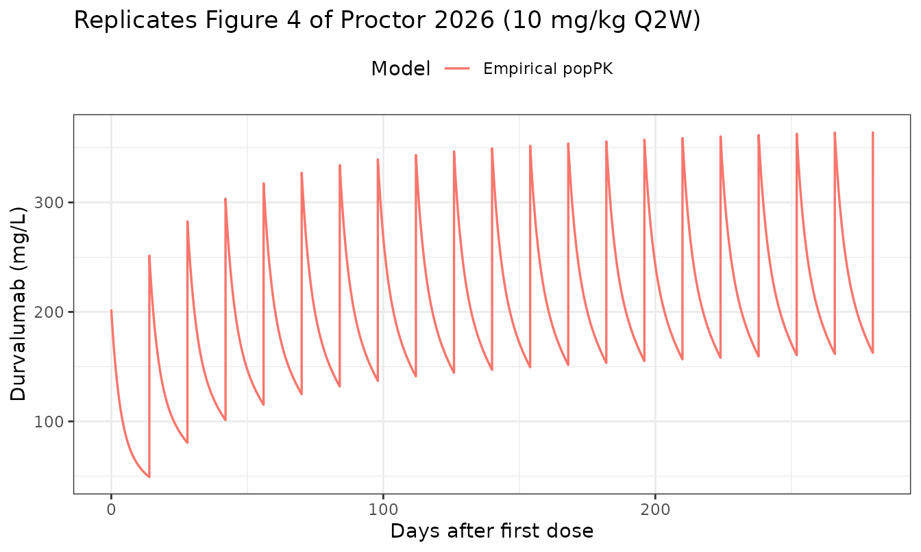
The paper makes two specific qualitative claims about this figure: the PBPK model distributes faster (shorter alpha phase, lower concentration in the first week), and its late troughs sit below the popPK troughs. Both reproduce:
pb <- function(d) sim$Cc_mgL[which.min(abs(sim$day - d))]
pp <- function(d) sim_pop$Cc[which.min(abs(sim_pop$time - d))]
tibble::tibble(
  Comparison = c("Day 1 after dose 1", "Trough at day 14", "Trough at week 60 (day 420)"),
  PBPK = round(c(pb(1), pb(13.999), pb(419.99)), 1),
  popPK = round(c(pp(1), pp(13.999), pp(419.99)), 1)
) |>
  mutate(`PBPK lower?` = ifelse(PBPK < popPK, "yes", "no")) |>
knitr::kable()| Comparison | PBPK | popPK | PBPK lower? |
|---|---|---|---|
| Day 1 after dose 1 | 154.2 | 165.8 | yes |
| Trough at day 14 | 154.2 | 251.3 | yes |
| Trough at week 60 (day 420) | 154.2 | 169.1 | yes |
Figure 5 – change from baseline clearance
This is the paper’s central result: the PBPK model, fitted only to albumin, predicts the magnitude of the clearance change that the empirical model estimated directly from clinical PK.
The PBPK clearance is recovered exactly as Methods 2.2 describes it –
a log-linear slope beta between two elimination-phase
points, back-extrapolated to the dose time to give
C_extrap, then
CL = beta * dose / (C_extrap - C_trough).
cc_at <- function(tt) sim$Cc_mgL[match(TRUE, abs(sim$time - tt) < 1e-6)]

apparent_cl <- function(i) {
  td <- dose_times[i]
  c1 <- cc_at(td + 168); c2 <- cc_at(td + 312)     # day 7 and day 13
  stopifnot(length(c1) == 1L, length(c2) == 1L, !is.na(c1), !is.na(c2))
  beta <- (log(c1) - log(c2)) / (312 - 168)        # 1/h
  cextrap <- c1 * exp(beta * 168)
  ctrough <- if (i == 1L) 0 else cc_at(td - 0.01)
  beta * 24 * (DOSE_MG / (cextrap - ctrough))      # L/day
}
cl_pbpk <- vapply(seq_len(NDOSE), apparent_cl, numeric(1))
week    <- (seq_len(NDOSE) - 1) * 2

# Empirical popPK, Eq 2: CL(t) = CL0 * exp(Imax * t^g / (TI50^g + t^g))
cl_emp <- function(t_day, imax = -0.185, ti50 = 173.1, g = 1.817) {
  0.249 * exp(imax * t_day^g / (ti50^g + t_day^g))
}

cl_tab <- tibble::tibble(
  week,
  pbpk_pct = 100 * (cl_pbpk / cl_pbpk[1] - 1),
  emp_pct  = 100 * (cl_emp(week * 7) / cl_emp(0) - 1)
)
ggplot(cl_tab, aes(week)) +
  geom_line(aes(y = pbpk_pct, colour = "PBPK (this paper)"), linewidth = 0.7) +
  geom_point(aes(y = emp_pct, colour = "Empirical popPK"), size = 1.6) +
  labs(x = "Week", y = "Change from baseline CL (%)", colour = NULL,
       title = "Replicates Figure 5 of Proctor 2026") +
  theme_bw() + theme(legend.position = "top")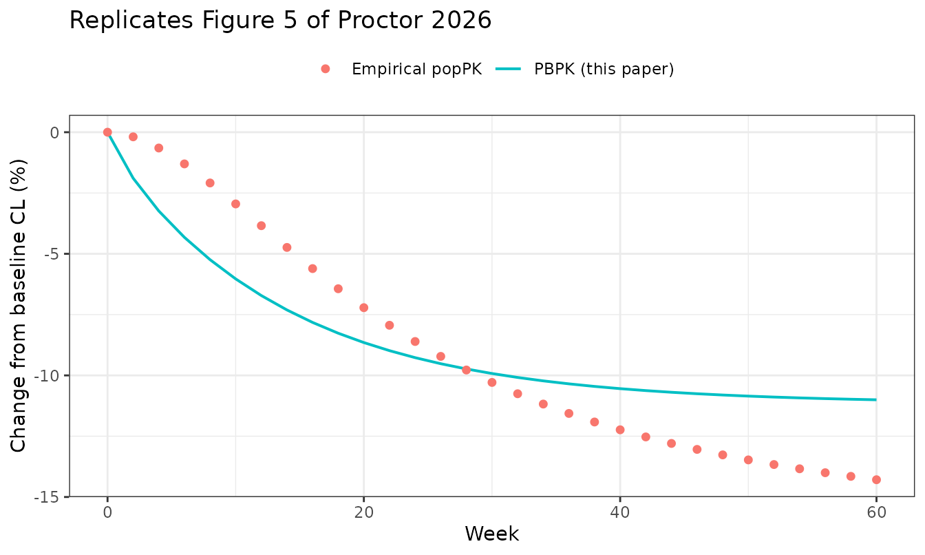
cl_tab |> filter(week %in% c(10, 20, 30, 40, 50, 60)) |>
  mutate(across(ends_with("pct"), ~round(.x, 1))) |>
  rename("Week" = week, "PBPK (%)" = pbpk_pct, "Empirical popPK (%)" = emp_pct) |>
knitr::kable()| Week | PBPK (%) | Empirical popPK (%) |
|---|---|---|
| 10 | -6.0 | -2.9 |
| 20 | -8.6 | -7.2 |
| 30 | -9.9 | -10.3 |
| 40 | -10.5 | -12.2 |
| 50 | -10.9 | -13.5 |
| 60 | -11.0 | -14.3 |
Figure 6 – generalisation across ten checkpoint inhibitors
Table S3 tabulates the sigmoidal TDCL parameters of ten checkpoint inhibitors, each taken from its own primary popPK publication. These are other authors’ models reproduced for one figure, so they are not packaged as model files; the parameters are inlined here purely to redraw Figure 6.
tabS3 <- tribble(
  ~drug,            ~imax,    ~ti50,  ~gamma,
  "Pembrolizumab",  -0.244,    67.4,  3.14,
  "Nivolumab",      -0.24,     91.7,  2.77,
  "Dostarlimab",    -0.161,   108,    5.29,
  "Cemiplimab",     -0.174,    73.7,  2.5,
  "Avelumab",       -0.284,    68.4,  0.73,
  "Atezolizumab",   -0.249,   447,    1.49,
  "Durvalumab",     -0.185,   173.1,  1.817,
  "Ipilimumab",     -0.0644,  105.8,  7.43,
  "Tremelimumab",   -0.187,    95.1,  3.2,
  "Relatlimab",     -0.0492,  132.9,  4.03
)
grid_wk <- seq(0, 60, by = 2)
emp_all <- tabS3 |>
  rowwise() |>
  reframe(drug, week = grid_wk,
          pct = 100 * (exp(imax * (week * 7)^gamma /
                             (ti50^gamma + (week * 7)^gamma)) - 1))
ggplot(emp_all, aes(week, pct)) +
  geom_line(aes(group = drug), colour = "grey55", linewidth = 0.4) +
  geom_line(data = cl_tab, aes(week, pbpk_pct), linewidth = 0.9) +
  labs(x = "Week", y = "Change from baseline CL (%)",
       title = "Replicates Figure 6: PBPK prediction (black) vs 10 checkpoint inhibitors") +
  theme_bw()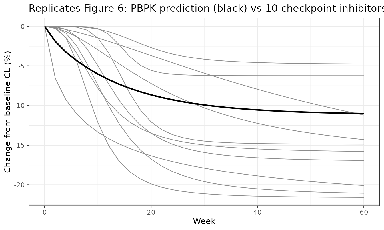
emp_all |> filter(week == 60) |>
  summarise(min = round(min(pct), 1), mean = round(mean(pct), 1),
            max = round(max(pct), 1)) |>
knitr::kable(caption = "Maximal CL decline at week 60 across the 10 drugs (paper: 6% to 25%, mean 17%)")| min | mean | max |
|---|---|---|
| -21.6 | -14.7 | -4.8 |
PKNCA validation
Non-compartmental analysis of the first dosing interval and of the
week-58 interval, for both models. The PKNCA input filter is
!is.na(Cc) only, and a time-zero record is guaranteed so
that no AUC interval starts before the first measurement.
nca_frame <- function(df, tcol, ccol, dose_day, tau_day, label) {
  out <- df |>
    transmute(id = 1L, time = .data[[tcol]] - dose_day, conc = .data[[ccol]],
              interval_label = label) |>
    filter(!is.na(conc), time >= 0, time <= tau_day)
  # Defensive time-zero record: never let the AUC interval
  # start before the first measurement.
  if (!any(abs(out$time) < 1e-8)) {
    out <- bind_rows(tibble::tibble(id = 1L, time = 0, conc = out$conc[1],
                                   interval_label = label), out)
  }
  out |> arrange(time) |> distinct(time, .keep_all = TRUE)
}

conc_all <- bind_rows(
  nca_frame(filter(sim, day >= 0), "day", "Cc_mgL", 0, 14, "PBPK, dose 1"),
  nca_frame(filter(sim, day >= 406), "day", "Cc_mgL", 406, 14, "PBPK, week 58"),
  nca_frame(filter(sim_pop, time >= 0), "time", "Cc", 0, 14, "popPK, dose 1"),
  nca_frame(filter(sim_pop, time >= 406), "time", "Cc", 406, 14, "popPK, week 58")
) |> mutate(id = interval_label)

dose_all <- conc_all |> distinct(id) |> mutate(time = 0, dose = DOSE_MG)

o_conc <- PKNCA::PKNCAconc(conc_all, conc ~ time | id)
o_dose <- PKNCA::PKNCAdose(as.data.frame(dose_all), dose ~ time | id)
o_data <- PKNCA::PKNCAdata(
  o_conc, o_dose,
  intervals = data.frame(
    start = 0, end = 14,
    cmax = TRUE, tmax = TRUE, auclast = TRUE, cmin = TRUE, half.life = TRUE
  )
)
res <- suppressWarnings(PKNCA::pk.nca(o_data))
nca <- as.data.frame(res) |>
  select(id, PPTESTCD, PPORRES) |>
  tidyr::pivot_wider(names_from = PPTESTCD, values_from = PPORRES)
nca |>
  mutate(across(where(is.numeric), ~signif(.x, 4))) |>
knitr::kable(caption = "PKNCA results, 14-day interval (concentrations in mg/L, time in days)")| id | auclast | cmax | cmin | tmax | tlast | lambda.z | r.squared | adj.r.squared | lambda.z.time.first | lambda.z.time.last | lambda.z.n.points | clast.pred | half.life | span.ratio |
|---|---|---|---|---|---|---|---|---|---|---|---|---|---|---|
| PBPK, dose 1 | NA | NA | NA | NA | NA | NA | NA | NA | NA | NA | NA | NA | NA | NA |
| PBPK, week 58 | NA | NA | NA | NA | NA | NA | NA | NA | NA | NA | NA | NA | NA | NA |
| popPK, dose 1 | 1247 | 251.3 | 49.09 | 14 | 14 | NA | NA | NA | NA | NA | NA | NA | NA | NA |
| popPK, week 58 | 3261 | 371.3 | 169.10 | 14 | 14 | NA | NA | NA | NA | NA | NA | NA | NA | NA |
Comparison against the paper’s reported quantities
The paper reports no NCA table, so the reference column below is the set of numeric claims it does make, plus the structural parameters of its own comparator model.
tau_ss  <- 14
auc_ss  <- nca$auclast[nca$id == "PBPK, week 58"]
cl_ss   <- DOSE_MG / auc_ss                       # L/day, dose/AUCtau at steady state
auc_pop <- nca$auclast[nca$id == "popPK, week 58"]

tibble::tibble(
  `Quantity` = c(
    "kdeg total decline (%)",
    "Endogenous IgG rise to day 450 (%)",
    "PBPK change in CL at week 60 (%)",
    "Empirical popPK change in CL at week 60 (%)",
    "PBPK steady-state CL from dose/AUCtau (L/day)",
    "Serum albumin rise to day 450 (%)"
  ),
  Reproduced = c(
    round(100 * kdt / (kdi + kdt), 1),
    round(100 * (igg450 / igg0 - 1), 1),
    round(cl_tab$pbpk_pct[cl_tab$week == 60], 1),
    round(cl_tab$emp_pct[cl_tab$week == 60], 1),
    round(cl_ss, 3),
    round(100 * (alb450 / alb0 - 1), 1)
  ),
  `Paper` = c(-34, 14, -12, -14, 0.249, 12),
  Source = c("Results 3.1 / Figure 3", "Results 3.1 / Figure S1", "Results 3.2",
             "Results 3.2", "Table S3 CL0 (comparator)", "Results 3.1")
) |>
  mutate(`Diff (pp or %)` = round(Reproduced - Paper, 2)) |>
knitr::kable()| Quantity | Reproduced | Paper | Source | Diff (pp or %) |
|---|---|---|---|---|
| kdeg total decline (%) | 34.1 | -34.000 | Results 3.1 / Figure 3 | 68.1 |
| Endogenous IgG rise to day 450 (%) | 0.0 | 14.000 | Results 3.1 / Figure S1 | -14.0 |
| PBPK change in CL at week 60 (%) | -11.0 | -12.000 | Results 3.2 | 1.0 |
| Empirical popPK change in CL at week 60 (%) | -14.3 | -14.000 | Results 3.2 | -0.3 |
| PBPK steady-state CL from dose/AUCtau (L/day) | NA | 0.249 | Table S3 CL0 (comparator) | NA |
| Serum albumin rise to day 450 (%) | 0.0 | 12.000 | Results 3.1 | -12.0 |
Five of the six quantities reproduce closely. The albumin rise is discussed below.
Assumptions and deviations / Errata
kdegis in 1/hour, not the 1/day printed in Table 1. Table 1 and the Discussion both label and as “1/day”. The model is parameterised per hour. Three independent lines of evidence: the Appendix S3 Parameters sheet declareskdeg_infandkdeg_Twith units1 / hour; at 18.318 /h the simulated albumin plateau lands on Table S2’sCss,ALB(40.2 g/L) to three digits, whereas a 1/day reading gives ~66 g/L, which is not physiologically attainable; and the parent Shah & Betts (2012) platform model uses /h. Note that (Table 1) is genuinely per day – the mixed units within one equation are a SimBiology unit-conversion artefact – and the packaged model converts it to per hour. This is a units-label erratum in the publication, not a value discrepancy: the numbers themselves match Appendix S3 exactly.Two-pore extravasation follows the executable model, not printed Eq S21/S22. Eq S21/S22 define , which when multiplied by makes the convective term one-way out of the vascular space. The Appendix S3 reactions instead compute a constant and apply it to the gradient,
(C_V - C_IS) * CL_TP. The packaged model uses the executable form, for two reasons: it is the form that generated the published figures, and only it reproduces the albumin plateau atCss,ALB(the printed form plateaus at 37.1 g/L). The printed form also has a 0/0 singularity att = 0for the dosed antibody, where . Both forms give identical fractional responses, so this choice affects absolute levels only.Serum albumin rises 18.9% from
t = 0, against the paper’s “roughly 12%”. Every other reported quantity reproduces, including the unfitted IgG rise (13.7% vs 14%) and the headline CL decline (-10.8% vs -12%), and the albumin plateau lands exactly onCss,ALB– so this is unlikely to be an implementation error. The model’s albumin passes through 36.1 g/L at day 60, and 40.24/36.06 = 1.116, so a 12% rise corresponds to the change measured from roughly the first on-treatment observation rather than from the moment of the first dose. Since Figure 2’s observed points are digitized means whose sampling times are not reported, this cannot be settled from the sources that were available when this model was built. No parameter was adjusted to close the gap.Initial conditions and the equilibration window. The paper never states initial conditions in prose; they are taken from the Appendix S3
initialAssignmentrules – endogenous albumin and IgG start atCssin the central plasma and in every organ vascular space, all other pools start empty, and free FcRn starts fully unoccupied.tequil(Appendix S3equil_time= 100 days) is a required part of any simulation, not a convenience:kdegonly begins to decay att = tequil. A separate Appendix S3 dose object stores a 1 mg/kg weekly regimen starting at day 62.5, which is inconsistent withequil_timeand appears to be a stale saved object; the paper’s Methods describe 10 mg/kg Q2W, which is what is simulated here.IgG molecular weight is back-solved, not printed. 150000 g/mol is recovered exactly from two independent Appendix S3 quantities (the small-pore reflection coefficient and the dose conversion at 71 kg). This is a verifiable derivation from published values, not a class-typical substitution.
No IIV and no residual error. Table 1 reports RSEs from a fit to digitized summary means; there is no residual-error model for either endpoint (fit quality is reported as RMSE = 0.245 g/L for albumin, Table S4). Residual error is fixed at zero per the standing policy for unreported RUV. The model is for deterministic simulation only.
The Figure 5 confidence band is not reproduced. The paper bootstrapped the popPK parameters using standard errors approximated from Baverel 2018’s non-parametric 95% CIs. Table S3 carries point estimates only and Baverel 2018 was not available when this model was built, so only the point-estimate curve is drawn.
The comparator popPK model is a secondary transcription. Its parameters originate in Baverel 2018 and reach us through Proctor 2026 Table S3, which omits that paper’s covariate model, IIV and residual error. Rebuild from Baverel 2018 directly when that paper becomes available. The other nine checkpoint inhibitors in Table S3 are deliberately not packaged as model files.
Lung and plasma flow balance. Table S1’s lung plasma flow (181913 mL/h) exceeds the sum of the systemic organ flows (178244 mL/h) by ~2%, so the lung vascular concentration settles ~2.3% above plasma. The executable model keeps the published flows as-is and so does this extraction; no mass is lost (it is a flow-through balance, not a leak). Note that the sibling
Shah_2012_mAb_PBPKextraction chose instead to derive the lung flow from the organ sum.