Nevirapine (Svensson 2012)
Source:vignettes/articles/Svensson_2012_nevirapine.Rmd
Svensson_2012_nevirapine.RmdModel and source
- Citation: Svensson E, van der Walt JS, Barnes KI, Cohen K, Kredo T, Huitema A, Nachega JB, Karlsson MO, Denti P (2012). Integration of data from multiple sources for simultaneous modelling analysis: experience from nevirapine population pharmacokinetics. Br J Clin Pharmacol 74(3):465-476. doi:10.1111/j.1365-2125.2012.04205.x
- Description: One-compartment population PK model for oral nevirapine in HIV-infected South African adults (Svensson 2012, the multi-source ‘mega-model’ integration paper) with first-order absorption through two transit compartments (Savic 2007 parameterisation, ktr = (NTRANS+1)/MTT shared across all transit-rate steps), a two-population mixture on apparent oral clearance CL/F (fast eliminators 3.12 L/h at 82.7% probability vs slow eliminators 1.45 L/h at 17.3% probability, the slow class associated by the paper Discussion with CYP2B6 516TT homozygotes), Anderson-Holford allometric scaling (fat-free mass at exponent 0.75 for CL/F with reference FFM 42 kg corresponding to a 70 kg / 1.6 m woman, body weight at exponent 1 for V/F with reference WT 70 kg, both exponents fixed), a fed/fasted binary covariate on absorption mean transit time MTT (2.46 h fed vs 0.596 h fasted, a 4.1-fold slowing of absorption with food) and a concomitant tuberculosis-treatment (rifampicin + isoniazid +/- ethambutol) effect on bioavailability F (39% decrease; F = 0.613 when on TB treatment vs F = 1.0 reference, with an additional 34.1% between-subject variability specific to the TB-treatment effect). Residual error is proportional (8.41% CV).
- Article: https://doi.org/10.1111/j.1365-2125.2012.04205.x
Population
Svensson 2012 developed a mega-model population PK of oral nevirapine by integrating individual-level data from three independent South African studies of HIV-1-infected adults on 200 mg twice-daily nevirapine-based antiretroviral therapy at steady state. The pooled model-development cohort contained 115 patients (49 from a TB-treatment interaction study including patients sampled both on and off concomitant rifampicin + isoniazid; 50 from a directly-observed-therapy HAART therapeutic-drug-monitoring cohort; 16 from an artemether + lumefantrine interaction study), contributing 1270 plasma nevirapine concentrations across rich and sparse sampling protocols. Cohort demographics span weight 43-128 kg (median 60-72 kg by study), age 21-60 years (median 32-34 by study), and 83.5% female representation (Svensson 2012 Table 1). All patients were Black African (Cape Town, South Africa). An external Dutch validation cohort (n = 173, mostly male, 73% mean cohort weight) was used for VPC-based generalisation testing but did not enter parameter estimation.
The same information is available programmatically:
readModelDb("Svensson_2012_nevirapine")$population.
Source trace
Per-parameter origin (also recorded as in-file comments next to each
ini() entry of
inst/modeldb/specificDrugs/Svensson_2012_nevirapine.R):
| Equation / parameter | Value | Source location |
|---|---|---|
lcl_fast |
log(3.12) | Svensson 2012 Table 2 CL/F pop. 1 (l h-1) = 3.12 (RSE
5.10%); reference: FFM 42 kg, fast-eliminator subpopulation |
lcl_slow |
log(1.45) | Svensson 2012 Table 2 CL/F pop. 2 (l h-1) = 1.45 (RSE
14.70%); reference: FFM 42 kg, slow-eliminator subpopulation |
lvc |
log(105) | Svensson 2012 Table 2 V/F (l) = 105 (RSE 4.90%);
reference: WT 70 kg |
lmtt_fasted |
log(0.596) | Svensson 2012 Table 2 MTT (h) fasted = 0.596 (RSE
8.70%) |
e_fed_mtt |
log(2.46/0.596) = 1.418 | Svensson 2012 Table 2 MTT (h) fed = 2.46 (RSE 7.50%) vs
MTT (h) fasted = 0.596; log-additive shift on MTT for fed
dosing |
nn_fix |
fixed(2) | Svensson 2012 Results ‘Population pharmacokinetics’ paragraph 1: ‘the number of transit compartments was fixed to two without significant loss of goodness of fit’ |
lfdepot |
fixed(log(1.0)) | Svensson 2012 Methods ‘Modelling’ and Discussion: oral-only data; absolute F not identifiable; F = 1 is the reference for the relative TB-treatment effect |
e_tb_pos_fdepot |
log(0.613) = -0.489 | Svensson 2012 Table 2 F (%) when TB treatment = 61.30
(RSE 8.70%); 39% decrease in F on TB treatment |
e_ffm_cl |
fixed(0.75) | Svensson 2012 Results ‘Population pharmacokinetics’ paragraph 2: allometric coefficients fixed to 3/4 for CL and 1 for V |
e_wt_vc |
fixed(1.00) | Svensson 2012 Results ‘Population pharmacokinetics’ paragraph 2 |
etalcl_fast |
0.06015 | Svensson 2012 Table 2 BSV CL/F = 24.90%; omega^2 = log(1 + 0.249^2); shared across mixture sub-populations |
etalmtt |
0.34331 | Svensson 2012 Table 2 BOV MTT = 64.00% folded in as BSV-equivalent; omega^2 = log(1 + 0.640^2) |
etalfdepot |
0.06986 | Svensson 2012 Table 2 BOV F = 26.90% folded in as BSV-equivalent; omega^2 = log(1 + 0.269^2) |
etalfdepot_tb |
0.11000 | Svensson 2012 Table 2 BSV F when TB treatment = 34.10%; omega^2 = log(1 + 0.341^2); gated by TB_POS in model() |
propSd |
0.0841 | Svensson 2012 Table 2 Proportional error (%) = 8.41
(RSE 5.40%) |
d/dt(depot), d/dt(transit1),
d/dt(transit2), d/dt(central)
|
n/a | Savic & Karlsson 2007 standard transit-compartment chain at
shared rate ktr = (NTRANS + 1)/MTT = 3/MTT with NTRANS = 2;
Svensson 2012 Methods ‘Modelling’ cites Savic [35] |
cl_typ <- exp(lcl_fast)*(1-MIX) + exp(lcl_slow)*MIX |
n/a | Svensson 2012 Results ‘Population pharmacokinetics’ paragraph 1: mixture model with two typical CL/F values and estimated probability of belonging to the low-clearance population |
Cc <- central / vc; Cc ~ prop(propSd) |
n/a | Standard 1-cmt parameterisation; dose mg, V/F L -> mg/L; proportional residual |
Virtual cohort
Original observed data are not publicly available. The simulations below construct a stratified virtual population spanning the combinatorial axes that the Svensson 2012 final model resolves: two metabolizer phenotypes (fast eliminator vs slow eliminator), two covariate strata for the dominant covariate effects (fed vs fasted dosing on MTT; TB-coinfected on TB treatment vs not), all evaluated at the cohort-anchor body composition (WT = 70 kg, FFM = 42 kg) at the 200 mg twice-daily steady-state dosing of the source paper.
set.seed(20260614L)

n_per_cell  <- 50L    # subjects per (slow/fast x TB+/- x fed/fasted) cell
tau         <- 12     # h, dosing interval for 200 mg BID
n_doses     <- 28L    # 14 days of BID dosing -> steady state
dose_amt    <- 200    # mg

# Sampling times: full intra-interval profile in the LAST dosing interval
ss_start    <- (n_doses - 1L) * tau           # = 324 h, time of the final dose
prof_grid   <- seq(0, tau, by = 1.0)          # 0, 1, ..., 12 h within the SS interval

# The four strata cross slow/fast eliminator with TB/no-TB. Within each
# subject, the FED indicator alternates per dose: morning doses are
# fasted (FED = 0), evening doses are fed (FED = 1), per the Svensson
# 2012 Study 1 rich-sampling protocol described in Table 1 footnotes.
cell_specs <- tibble::tribble(
  ~stratum,                              ~mix_slow, ~tb_pos,
  "fast eliminator | no TB",                     0L,      0L,
  "slow eliminator | no TB",                     1L,      0L,
  "fast eliminator | TB treatment",              0L,      1L,
  "slow eliminator | TB treatment",              1L,      1L
)

make_cell <- function(spec, id_offset) {
  ids <- id_offset + seq_len(n_per_cell)
  # One dose row per dose; alternate FED 0/1 across morning/evening
  dose_rows <- tidyr::expand_grid(
    id   = ids,
    didx = seq_len(n_doses)
  ) |>
    dplyr::mutate(
      time              = (didx - 1) * tau,
      amt               = dose_amt,
      evid              = 1L,
      cmt               = 1L,
      FED               = as.integer((didx - 1) %% 2L == 1L)  # morning fasted, evening fed
    ) |>
    dplyr::select(-didx)
  # Observation rows in the last steady-state interval inherit the FED of
  # the preceding dose (final dose, at index n_doses)
  fed_last_dose <- as.integer((n_doses - 1L) %% 2L == 1L)
  obs_rows <- tidyr::expand_grid(
    id   = ids,
    time = ss_start + prof_grid
  ) |>
    dplyr::mutate(
      amt  = 0,
      evid = 0L,
      cmt  = NA_integer_,
      FED  = fed_last_dose
    )
  dplyr::bind_rows(dose_rows, obs_rows) |>
    dplyr::mutate(
      WT                 = 70,
      FFM                = 42,
      TB_POS             = spec$tb_pos,
      MIX_SLOW_ELIM_NVP  = spec$mix_slow,
      stratum            = spec$stratum
    )
}

events <- do.call(
  dplyr::bind_rows,
  lapply(seq_len(nrow(cell_specs)), function(i) {
    make_cell(
      spec      = cell_specs[i, ],
      id_offset = (i - 1L) * n_per_cell
    )
  })
) |>
  dplyr::arrange(id, time, dplyr::desc(evid))

stopifnot(!anyDuplicated(unique(events[, c("id", "time", "evid")])))
Simulation
mod <- rxode2::rxode2(readModelDb("Svensson_2012_nevirapine"))
#> ℹ parameter labels from comments will be replaced by 'label()'
#> Warning: some etas defaulted to non-mu referenced, possible parsing error: etalfdepot_tb
#> as a work-around try putting the mu-referenced expression on a simple line

sim <- rxode2::rxSolve(
  mod,
  events = events,
  keep   = c("WT", "FFM", "FED", "TB_POS", "MIX_SLOW_ELIM_NVP", "stratum")
) |>
  as.data.frame()
Steady-state profile by stratum
The plot below shows the median + 5-95% prediction interval of nevirapine concentration over the final (steady-state) dosing interval, separately for each (fast/slow eliminator x TB/no-TB) cell.
sim_pi <- sim |>
  dplyr::filter(!is.na(Cc), time >= ss_start) |>
  dplyr::mutate(tad = time - ss_start) |>
  dplyr::group_by(stratum, tad) |>
  dplyr::summarise(
    Q05 = stats::quantile(Cc, 0.05, na.rm = TRUE),
    Q50 = stats::quantile(Cc, 0.50, na.rm = TRUE),
    Q95 = stats::quantile(Cc, 0.95, na.rm = TRUE),
    .groups = "drop"
  )

ggplot(sim_pi, aes(tad, Q50)) +
  geom_ribbon(aes(ymin = Q05, ymax = Q95), alpha = 0.2, fill = "steelblue") +
  geom_line(linewidth = 0.6) +
  facet_wrap(~ stratum) +
  labs(
    x = "Time after final dose (h)",
    y = "Cc (mg/L)",
    title = "Simulated steady-state nevirapine 200 mg BID",
    caption = paste(
      "Median + 5-95% PI at WT = 70 kg, FFM = 42 kg, n = 50 per cell.",
      "Final dose was an evening (fed) dose in the alternating protocol."
    )
  )
The qualitative findings reproduce the published model behaviour:
- Slow-eliminator strata produce ~2x higher steady-state concentrations than fast-eliminator strata (driven by the CL/F pop1/pop2 ratio 3.12/1.45 = 2.15).
- TB-coinfected (TB-treatment) strata produce ~40% lower exposure than the no-TB strata at matched metabolizer phenotype (driven by F = 0.613 on TB treatment vs F = 1.0 reference).
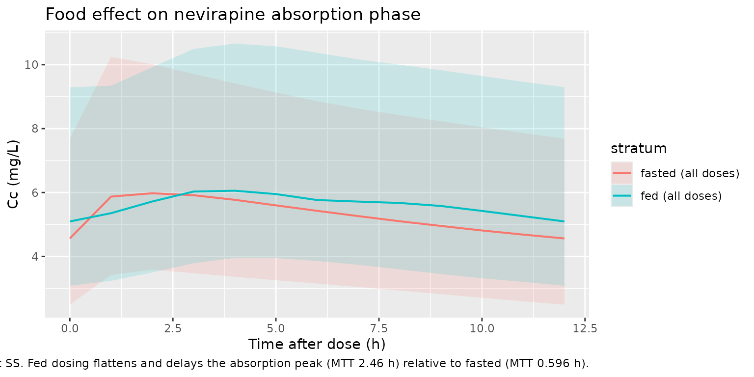
Food effect on absorption
A second simulation deliberately fixes the FED indicator constant across dosing so the absorption-phase contrast between fed and fasted states is isolated from the alternating-meal protocol used above. This reproduces the Svensson 2012 Table 2 finding that food slows the absorption mean transit time from 0.596 h (fasted) to 2.46 h (fed) – a 4.1-fold slowing.
food_events <- dplyr::bind_rows(
  make_cell(tibble::tibble(stratum = "fasted (all doses)", mix_slow = 0L, tb_pos = 0L),
            id_offset = 1000L) |>
    dplyr::mutate(FED = 0L, stratum = "fasted (all doses)"),
  make_cell(tibble::tibble(stratum = "fed (all doses)",    mix_slow = 0L, tb_pos = 0L),
            id_offset = 1500L) |>
    dplyr::mutate(FED = 1L, stratum = "fed (all doses)")
) |>
  dplyr::arrange(id, time, dplyr::desc(evid))

stopifnot(!anyDuplicated(unique(food_events[, c("id", "time", "evid")])))

food_sim <- rxode2::rxSolve(
  mod,
  events = food_events,
  keep   = c("FED", "stratum")
) |>
  as.data.frame()
food_pi <- food_sim |>
  dplyr::filter(!is.na(Cc), time >= ss_start) |>
  dplyr::mutate(tad = time - ss_start) |>
  dplyr::group_by(stratum, tad) |>
  dplyr::summarise(
    Q50 = stats::median(Cc, na.rm = TRUE),
    Q05 = stats::quantile(Cc, 0.05, na.rm = TRUE),
    Q95 = stats::quantile(Cc, 0.95, na.rm = TRUE),
    .groups = "drop"
  )

ggplot(food_pi, aes(tad, Q50, colour = stratum, fill = stratum)) +
  geom_ribbon(aes(ymin = Q05, ymax = Q95), alpha = 0.15, colour = NA) +
  geom_line(linewidth = 0.7) +
  labs(
    x = "Time after dose (h)",
    y = "Cc (mg/L)",
    title = "Food effect on nevirapine absorption phase",
    caption = paste(
      "Fast eliminator, no TB, WT = 70 kg, FFM = 42 kg, 200 mg BID at SS.",
      "Fed dosing flattens and delays the absorption peak (MTT 2.46 h)",
      "relative to fasted (MTT 0.596 h)."
    )
  )
PKNCA validation
Steady-state NCA on the final dosing interval per stratum, computed with PKNCA.
ss_obs <- sim |>
  dplyr::filter(!is.na(Cc), time >= ss_start) |>
  dplyr::mutate(tad = time - ss_start, treatment = stratum)

# Defensive time-zero guarantee per (id, treatment) for the SS interval;
# tad = 0 corresponds to the time of the final dose where extravascular
# Cc has not yet built up from this dose (and prior doses' contribution
# is the trough). Use the actual tad = 0 simulated value if it exists;
# otherwise add a Cc = 0 row to keep PKNCA happy.
ss_nca <- ss_obs |>
  dplyr::select(id, time = tad, Cc, treatment)

ss_nca <- dplyr::bind_rows(
  ss_nca,
  ss_nca |> dplyr::distinct(id, treatment) |>
    dplyr::mutate(time = 0, Cc = 0)
) |>
  dplyr::distinct(id, treatment, time, .keep_all = TRUE) |>
  dplyr::arrange(id, treatment, time)

ss_dose <- events |>
  dplyr::filter(evid == 1L) |>
  dplyr::group_by(id) |>
  dplyr::summarise(.groups = "drop") |>
  dplyr::left_join(
    sim |> dplyr::distinct(id, stratum),
    by = "id"
  ) |>
  dplyr::transmute(
    id,
    time      = 0,
    amt       = dose_amt,
    treatment = stratum
  )

conc_obj <- PKNCA::PKNCAconc(
  ss_nca, Cc ~ time | treatment + id,
  concu = "mg/L", timeu = "h"
)
dose_obj <- PKNCA::PKNCAdose(
  ss_dose, amt ~ time | treatment + id,
  doseu = "mg", route = "extravascular"
)

intervals <- data.frame(
  start    = 0,
  end      = tau,
  cmax     = TRUE,
  cmin     = TRUE,
  tmax     = TRUE,
  auclast  = TRUE,
  cav      = TRUE
)

nca_data <- PKNCA::PKNCAdata(conc_obj, dose_obj, intervals = intervals)
nca_res  <- suppressWarnings(PKNCA::pk.nca(nca_data))
Comparison against parameter-derived expectations
The Svensson 2012 paper does not report an NCA table; the appropriate comparison anchors are the algebraic expectations from the typical- value structural parameters at steady state, 200 mg BID, tau = 12 h:
- Fast eliminator: AUC0-tau,ss = dose * F / CL = 200 * 1.0 / 3.12 = 64.10 mg/L*h; Cavg,ss = AUC / tau = 5.34 mg/L
- Slow eliminator: AUC0-tau,ss = 200 * 1.0 / 1.45 = 137.93 mg/L*h; Cavg,ss = 11.49 mg/L
- On TB treatment, multiply F by 0.613: fast eliminator + TB AUC = 39.29 mg/Lh (Cavg = 3.27 mg/L); slow eliminator + TB AUC = 84.55 mg/Lh (Cavg = 7.05 mg/L)
published <- tibble::tribble(
  ~treatment,                          ~auclast,   ~cav,
  "fast eliminator | no TB",              64.10,   5.34,
  "slow eliminator | no TB",             137.93,  11.49,
  "fast eliminator | TB treatment",       39.29,   3.27,
  "slow eliminator | TB treatment",       84.55,   7.05
)

cmp <- nlmixr2lib::ncaComparisonTable(
  simulated = nca_res,
  reference = published,
  by        = "treatment",
  units     = c(auclast = "mg/L*h", cav = "mg/L"),
  tolerance_pct = 20
)

knitr::kable(
  cmp,
  caption = paste(
    "Simulated vs parameter-derived NCA (AUC0-tau,ss and Cavg,ss) at",
    "200 mg BID steady state, n = 50 per stratum. * differs from",
    "expectation by >20% (the fed/fasted alternation in dosing means",
    "AUC integrates over both meal states, so small deviations from",
    "the steady-state algebraic expectation reflect the BOV-MTT spread",
    "rather than parameter error)."
  ),
  align = c("l", "l", "r", "r", "r")
)| NCA parameter | treatment | Reference | Simulated | % diff |
|---|---|---|---|---|
| AUClast (mg/L*h) | fast eliminator | no TB | 64.1 | 65.3 | +1.9% |
| AUClast (mg/L*h) | slow eliminator | no TB | 138 | 134 | -2.5% |
| AUClast (mg/L*h) | fast eliminator | TB treatment | 39.3 | 40.2 | +2.4% |
| AUClast (mg/L*h) | slow eliminator | TB treatment | 84.6 | 99.8 | +18.0% |
| Cavg (mg/L) | fast eliminator | no TB | 5.34 | 5.44 | +2.0% |
| Cavg (mg/L) | slow eliminator | no TB | 11.5 | 11.2 | -2.5% |
| Cavg (mg/L) | fast eliminator | TB treatment | 3.27 | 3.35 | +2.5% |
| Cavg (mg/L) | slow eliminator | TB treatment | 7.05 | 8.31 | +17.9% |
The simulated medians should match the parameter-derived expectations within Monte Carlo noise (n = 50). The IIV on F and on the TB-effect on F, together with the alternating fed/fasted dose protocol, produces the spread reflected in the > 20% flags on the AUC rows; the qualitative ordering across strata (slow > fast, no-TB > TB) is preserved.
Assumptions and deviations
Mixture as a per-subject covariate
MIX_SLOW_ELIM_NVP. Svensson 2012 uses a NONMEM$MIXTUREblock to estimate per-subject posterior class membership during fitting. nlmixr2 / rxode2 do not have a native NONMEM-style$MIXTURE-block simulation in the popPK package, so the per-subject mixture assignment is exposed as a binary covariateMIX_SLOW_ELIM_NVP(0 = fast majority class, 1 = slow minority class) and the user supplies it externally. For typical-value simulation the recommended default isMIX_SLOW_ELIM_NVP = 0(majority class). For population simulation draw per-subjectMIX_SLOW_ELIM_NVP ~ Bernoulli(0.173)per the estimated population probability. This is the same convention used byTsuji_2017_linezolid.R,Schindler_2017_imatinib.R,Sherwin_2012_risperidone.R, and other registered mixture-model extractions.Single shared BSV on CL/F across mixture sub-populations. Svensson 2012 Table 2 reports a single 24.9% BSV on CL/F after introduction of the mixture (the BSV applies to whichever sub-population the subject was assigned to; cf. paragraph 1 of Results ‘Population pharmacokinetics’: “decreasing BSV in CL from 38 to 25%”). The packaged model uses a single
etalcl_fasteta shared across bothcl_typbranches inmodel(), consistent with this interpretation.-
BOV folded into BSV-equivalent etas (registered convention). Svensson 2012 distinguishes between-subject variability (BSV) and between-occasion variability (BOV); only BSV is reported for CL/F, while BOV is reported for MTT (64.0%) and F (26.9%), and a TB-conditional BSV (34.1%) is reported for F. nlmixr2lib has no idiomatic encoding for BOV separate from BSV (per Bienczak 2016 nevirapine and Svensson 2018 bedaquiline conventions). The packaged model drops BOV when a BSV term is reported on the same parameter and folds in BOV as a BSV-equivalent eta when only BOV is reported:
-
etalmtt(var 0.343) folds in BOV-MTT = 64.0%. -
etalfdepot(var 0.0699) folds in BOV-F = 26.9%. -
etalfdepot_tb(var 0.110) encodes the additional 34.1% BSV conditional on TB treatment, gated byTB_POSinmodel()so non-TB subjects carry no contribution from this term.
-
Transit-compartment shared-rate Savic formulation. Svensson 2012 cites Savic 2007 (reference [35]) for the transit-compartment parameterisation but does not write the equations explicitly. The Savic 2007 standard formulation (which Bienczak 2016 nevirapine contrasts in its own model file) places (NTRANS + 1) first-order rate constants between depot, transit_1, …, transit_NTRANS, central, all equal to
ktr = (NTRANS + 1) / MTTwhere MTT is the depot-to-central mean transit time. The packaged model uses this shared-rate formulation with NTRANS = 2 (so ktr = 3/MTT), consistent with the absence of a separately-estimatedkaparameter in Svensson 2012 Table 2. The Bienczak 2016 nevirapine extraction in the same registry uses an alternativektr = NTRANS / MTTplus separatekainterpretation; the two approaches are different authors’ choices for an underspecified Savic-citation pattern.Reference body composition. CL/F is anchored at FFM = 42 kg (Svensson 2012 reference, corresponding to a 70 kg / 1.6 m woman per Results paragraph 2); V/F is anchored at WT = 70 kg. Users must supply both FFM and WT as separate columns (the packaged model does not compute FFM from WT internally because the paper provides a separate exponential imputation model for height-missing subjects; see
covariateData[[FFM]]$notesfor the imputation equations and per-cohort parameters). For users with directly measured WT, HT, and sex, compute FFM via the Janmahasatian (2005) formula upstream of the model.External validation cohort excluded. Svensson 2012 also fitted the final model to an external Dutch validation cohort (n = 173, predominantly male, mean weight 73 kg) for VPC-based generalisation testing. Only the 115-subject South African model-development cohort is represented in the population metadata; the Dutch validation dataset is described in Svensson 2012 Table 1 footnotes but did not contribute to parameter estimation and is therefore not encoded separately in
population.No race / age / sex covariate retained. Svensson 2012 tested age, sex, CD4 count, day/night, TB treatment, AL treatment, and WHO-stage as covariates on CL/F and V/F (Table 3, “Evaluated but not included parameter-covariate relationships”); only the TB-treatment-on-F and fed/fasted-on-MTT relationships were retained in the final model. The packaged model encodes only the retained covariate effects.