Mobocertinib, AP32960 and AP32914 (Gupta 2022)
Source:vignettes/articles/Gupta_2022_mobocertinib.Rmd
Gupta_2022_mobocertinib.RmdModel and source
- Citation: Gupta N, Pierrillas PB, Hanley MJ, Zhang S, Diderichsen PM (2022). Population pharmacokinetics of mobocertinib in healthy volunteers and patients with non-small cell lung cancer. CPT Pharmacometrics Syst Pharmacol 11(6):731-744. doi:10.1002/psp4.12785. Structure from the final NONMEM control stream (Supporting Information, supplementary data file ‘Final model control stream’); parameter values from Table 3.
- Description: Joint semimechanistic population PK model for oral mobocertinib (an irreversible EGFR exon 20 insertion tyrosine kinase inhibitor) and its two active metabolites AP32960 and AP32914 in healthy adult volunteers and adults with metastatic non-small cell lung cancer. Mobocertinib is absorbed from the depot through three transit compartments (transit rate equal to ka) into a two-compartment disposition model. Its clearance forms AP32960 (fixed fraction 0.62, two-compartment disposition) and AP32914 (fixed fraction 0.08, one-compartment disposition), and the remaining 0.30 is eliminated. Auto-induction is a turnover enzyme pool whose production rate is stimulated by an Emax function of the molar sum of the three plasma concentrations; the relative enzyme amount multiplies the clearances of all three moieties. Healthy-volunteer status raises the mobocertinib central volume and all three clearances. Amounts are in umol and concentrations in umol/L.
- Article: CPT Pharmacometrics Syst Pharmacol 2022;11(6):731-744 (open access)
Mobocertinib is an oral, irreversible tyrosine kinase inhibitor for metastatic non-small cell lung cancer (mNSCLC) with EGFR exon 20 insertion mutations. The recommended dose is 160 mg once daily. CYP3A converts it by dealkylation to two active metabolites, AP32960 and AP32914, which are about as potent against EGFR as the parent. All three moieties are CYP3A substrates and inducers. On repeat dosing, exposure accumulates less than the single-dose half-life predicts, which points to auto-induction.
The final model is a joint semimechanistic model of the three moieties (Figure 1 of the paper):
- The dose enters a depot and passes through three transit compartments to the mobocertinib central compartment. All four rate constants equal ka.
- Mobocertinib has two-compartment disposition. Of its clearance, a fixed molar fraction of 0.62 forms AP32960, 0.08 forms AP32914, and the remaining 0.30 leaves the system.
- AP32960 has two-compartment disposition and AP32914 one-compartment disposition.
- An enzyme pool starts at 1. Its production rate is stimulated by an
Emax function of the molar sum of the three plasma concentrations:
d(enzyme)/dt = kenz * (1 + Emax * C / (EC50 + C)) - kenz * enzyme. The enzyme amount multiplies all three clearances. - Healthy volunteers have a larger mobocertinib central volume and higher clearances of all three moieties than patients.
The model runs in molar units, as the authors fitted it. Doses are in umol and concentrations in umol/L. Doses are converted from mg with the free-base molecular weight of mobocertinib, 585.7 g/mol (C32H39N7O4; PubChem CID 118607832). The paper does not give the metabolite molecular weights, so metabolite concentrations are reported in nM only.
Population
The analysis pooled 427 participants from four studies (Tables 1 and 2):
- 297 patients from the global phase I/II study (NCT02716116). Doses were 5-180 mg once daily or 40-60 mg twice daily, with 160 mg once daily in the expansion and extension cohorts.
- 20 Japanese patients from the phase I part of a phase I/II study (NCT03807778), at 40, 120 or 160 mg once daily.
- 86 healthy volunteers from a single-rising-dose, food-effect and relative bioavailability study (NCT03482453), at single doses of 20-160 mg.
- 24 healthy volunteers from the periods without a CYP3A modulator in a drug-drug interaction study (NCT03928327), at single doses of 20 or 160 mg.
So 317 participants (74.2%) were patients with mNSCLC and 110 (25.8%) were healthy volunteers. Mean age was 52.9 years (SD 17.0; range 18-86) and mean body weight 70.4 kg (SD 15.9; range 37.3-132). 57.1% were female. 66.3% were White, 26.9% Asian and 4.4% Black. The dataset held 5880 mobocertinib, 5880 AP32960 and 5879 AP32914 post-dose concentrations (Supporting Information Table S1).
The same information is available programmatically:
str(readModelDb("Gupta_2022_mobocertinib")()$population)
#> List of 11
#>  $ species       : chr "human"
#>  $ n_subjects    : int 427
#>  $ n_studies     : int 4
#>  $ age_range     : chr "18-86 years (mean 52.9, SD 17.0; Table 2)"
#>  $ weight_range  : chr "37.3-132 kg (mean 70.4, SD 15.9; Table 2)"
#>  $ sex_female_pct: num 57.1
#>  $ race_ethnicity: Named num [1:5] 66.3 26.9 4.4 0.2 2.1
#>   ..- attr(*, "names")= chr [1:5] "White" "Asian" "Black" "American Indian/Alaskan native" ...
#>  $ disease_state : chr "317 adults with metastatic non-small cell lung cancer (EGFR or HER2 mutations; 289 with at least one prior trea"| __truncated__
#>  $ dose_range    : chr "Patients: 5-180 mg once daily or 40-60 mg twice daily (recommended dose 160 mg once daily); healthy volunteers:"| __truncated__
#>  $ regions       : chr "Global phase I/II study (NCT02716116), Japanese phase I/II study (NCT03807778), and two phase I healthy-volunte"| __truncated__
#>  $ notes         : chr "5880 mobocertinib, 5880 AP32960 and 5879 AP32914 post-dose observations (Supporting Information Table S1). BLQ "| __truncated__
Source trace
The Supporting Information includes the complete NONMEM control
stream of the final model. It fixes the model structure, the fixed
metabolite fractions, the molar units, and the linear form of the
healthy-volunteer effects. Its $THETA and
$OMEGA records are not printed. The parameter values come
from Table 3, using the “Untransformed parameter” column, which has one
more significant figure than the log-scale “Estimate” column.
| Equation / parameter | Value | Source location |
|---|---|---|
lka (ka = ktr) |
2.12 /h | Table 3; control stream KTR = KA
|
lvc (Vc/F, patients) |
2340 L | Table 3 |
lcl (CL/F, patients) |
108 L/h | Table 3 |
lq (Q/F) |
11.7 L/h | Table 3 |
lvp (Vp/F) |
1110 L | Table 3 |
fm_ap32960 |
0.62, fixed | Methods; control stream FM60 = 0.62
|
fm_ap32914 |
0.08, fixed | Methods; control stream FM14 = 0.08
|
lcl_ap32960 (CL/F, patients) |
117 L/h | Table 3 |
lvc_ap32960 |
12.8 L | Table 3 |
lq_ap32960 |
26.5 L/h | Table 3 |
lvp_ap32960 |
1090 L | Table 3 |
lcl_ap32914 (CL/F, patients) |
124 L/h | Table 3 |
lvc_ap32914 |
30.6 L | Table 3 |
e_healthy_vc |
0.787 | Table 3; control stream V2HV = 1 + THETA(18)
|
e_healthy_cl |
0.900 | Table 3; control stream CLHV = 1 + THETA(15)
|
e_healthy_cl_ap32960 |
0.738 | Table 3; control stream CLM60HV = 1 + THETA(17)
|
e_healthy_cl_ap32914 |
0.909 | Table 3; control stream CLM14HV = 1 + THETA(16)
|
lkenz |
0.00392 /h | Table 3 |
lec50 |
213 nM = 0.213 umol/L | Table 3 |
lemax |
0.781 | Table 3 |
etalka |
0.209 | Table 3 omega^2 |
etalvc, etalcl,
etalcl_ap32960, etalcl_ap32914 block |
variances 0.237, 0.246, 0.157, 0.295; six covariances | Table 3 omega^2 and covariance rows |
expSd, expSd_ap32960,
expSd_ap32914
|
0.414, 0.373, 0.405 | Table 3; control stream Y = LOG(C) + THETA*EPS,
$SIGMA 1 FIX
|
d/dt(depot), d/dt(transit1..3)
|
n/a | control stream DADT(1),
DADT(6)-DADT(8); Figure 1 |
d/dt(central), d/dt(peripheral1)
|
n/a | control stream DADT(2), DADT(3)
|
d/dt(central_ap32960),
d/dt(peripheral1_ap32960)
|
n/a | control stream DADT(4), DADT(9)
|
d/dt(central_ap32914) |
n/a | control stream DADT(5)
|
d/dt(enzyme), enzyme(0) <- 1,
c_molar_sum
|
n/a | control stream DADT(10), A_0(10) = 1,
CTOT = C2 + C4 + C5
|
Cc, Cc_ap32960, Cc_ap32914
(umol/L) |
n/a | control stream $ERROR (‘concentration in uM’) |
Helpers
mw_mobo <- 585.7 # g/mol, mobocertinib free base (PubChem CID 118607832)
mg_to_umol <- function(mg) mg / mw_mobo * 1000

mod <- readModelDb("Gupta_2022_mobocertinib")
mod_typical <- rxode2::zeroRe(mod)
#> ℹ parameter labels from comments will be replaced by 'label()'

# The model has three declared endpoints and no state endpoint, so observation
# rows are keyed by dvid with cmt left empty; rxode2 then returns Cc,
# Cc_ap32960 and Cc_ap32914 on every observation row. Doses go to the depot.
make_events <- function(ids, dose_mg, n_doses, obs_times, covs) {
  dose_rows <- data.frame(
    id = ids, time = 0, evid = 1L, amt = mg_to_umol(dose_mg),
    cmt = "depot", ii = 24, addl = n_doses - 1L, dvid = NA_integer_
  )
  obs_rows <- expand.grid(id = ids, time = obs_times) |>
    dplyr::mutate(
      evid = 0L, amt = 0, cmt = NA_character_, ii = 0, addl = 0L, dvid = 1L
    )
  dplyr::bind_rows(dose_rows, obs_rows) |>
    dplyr::left_join(covs, by = "id") |>
    dplyr::arrange(id, time, dplyr::desc(evid))
}

auc_trap <- function(time, conc) {
  sum(diff(time) * (head(conc, -1) + tail(conc, -1)) / 2)
}

# Concentrations in nM; the molar sum is the exposure metric of the paper.
add_nm <- function(sim) {
  sim |>
    dplyr::mutate(
      Mobocertinib = Cc * 1000,
      AP32960 = Cc_ap32960 * 1000,
      AP32914 = Cc_ap32914 * 1000,
      `Molar sum` = Mobocertinib + AP32960 + AP32914
    )
}
Typical-value checks
Steady-state molar-sum Cmax and metabolite shares
The paper states that the typical molar-sum Cmax at steady state after 160 mg once daily is 214 nM, close to the EC50 of 213 nM (Results). The enzyme pool has a half-life of log(2) / 0.00392 = 177 h, so induction takes about five weeks to complete. The check below uses the 60th daily dose, when induction is complete.
The US prescribing information (reference 14 of the paper) gives AP32960 and AP32914 as 36% and 4% of the combined molar AUC. That figure comes from the clinical studies rather than the model, so it is a looser check of the fixed metabolite fractions and the metabolite clearances.
covs_typ <- data.frame(id = 1:2, DIS_HEALTHY = c(0L, 1L))
obs_typ <- sort(unique(c(
  seq(0, 24, by = 0.1), seq(672, 696, by = 0.1), seq(1416, 1440, by = 0.1),
  seq(0, 1440, by = 2)
)))
ev_typ <- make_events(
  ids = covs_typ$id, dose_mg = 160, n_doses = 60L,
  obs_times = obs_typ, covs = covs_typ
)
sim_typ <- rxode2::rxSolve(
  mod_typical, events = ev_typ, keep = "DIS_HEALTHY", useLinCmt = FALSE
) |>
  as.data.frame() |>
  add_nm()
#> ℹ omega/sigma items treated as zero: 'etalka', 'etalvc', 'etalcl', 'etalcl_ap32960', 'etalcl_ap32914'
#> Warning: multi-subject simulation without without 'omega'

ss_pat <- dplyr::filter(sim_typ, id == 1, time >= 1416)
cmax_sum_ss <- max(ss_pat$`Molar sum`)
auc_ss <- sapply(
  c("Mobocertinib", "AP32960", "AP32914", "Molar sum"),
  function(a) auc_trap(ss_pat$time, ss_pat[[a]])
)
share <- auc_ss[c("AP32960", "AP32914")] / auc_ss[["Molar sum"]]

data.frame(
  Quantity = c(
    "Molar-sum Cmax at steady state (nM)", "Tmax of mobocertinib (h)",
    "AP32960 share of molar AUC (%)", "AP32914 share of molar AUC (%)",
    "Enzyme amount at steady state (fold baseline)"
  ),
  Published = c("214", "4-6 (single dose)", "36", "4", "not reported"),
  Model = c(
    sprintf("%.1f", cmax_sum_ss),
    sprintf("%.1f", ss_pat$time[which.max(ss_pat$Mobocertinib)] - 1416),
    sprintf("%.1f", 100 * share[["AP32960"]]),
    sprintf("%.1f", 100 * share[["AP32914"]]),
    sprintf("%.2f", max(ss_pat$enzyme))
  )
) |>
knitr::kable(caption = "Typical patient, 160 mg once daily, 60th dose.")| Quantity | Published | Model |
|---|---|---|
| Molar-sum Cmax at steady state (nM) | 214 | 213.0 |
| Tmax of mobocertinib (h) | 4-6 (single dose) | 3.7 |
| AP32960 share of molar AUC (%) | 36 | 34.9 |
| AP32914 share of molar AUC (%) | 4 | 4.2 |
| Enzyme amount at steady state (fold baseline) | not reported | 1.29 |
stopifnot(
  # The typical value is deterministic, so this bound is tight.
  abs(cmax_sum_ss / 214 - 1) < 0.03,
  abs(100 * share[["AP32960"]] - 36) < 3,
  abs(100 * share[["AP32914"]] - 4) < 1
)
The steady-state Cmax matches the paper. It depends on every part of the model at once: the absorption chain, the parent and metabolite clearances, the fixed metabolite fractions, the induction loop, and the molar units. EC50 is in nM, so a wrong reading of the concentration unit would move the steady-state enzyme level, and with it Cmax, by a large factor.
Typical profiles (Supporting Information Figure S1)
# Typical-value profiles on the time scale of Supporting Information Figure S1
# of Gupta 2022 (cycle 1 day 1 and cycle 2 day 1).
sim_typ |>
  dplyr::filter(time <= 24 | (time >= 672 & time <= 696)) |>
  dplyr::mutate(
    day = ifelse(time <= 24, "Cycle 1, day 1", "Cycle 2, day 1"),
    tad = ifelse(time <= 24, time, time - 672),
    group = ifelse(DIS_HEALTHY == 1, "Healthy volunteer", "Patient with mNSCLC")
  ) |>
  tidyr::pivot_longer(
    c(Mobocertinib, AP32960, AP32914),
    names_to = "analyte", values_to = "conc_nM"
  ) |>
  dplyr::filter(tad > 0) |>
  dplyr::mutate(analyte = factor(analyte, levels = c("Mobocertinib", "AP32960", "AP32914"))) |>
  ggplot(aes(tad, conc_nM, colour = group)) +
  geom_line() +
  facet_grid(day ~ analyte) +
  scale_y_log10() +
  labs(
    x = "Time after dose (h)", y = "Concentration (nM)", colour = NULL,
    title = "Typical profiles, 160 mg once daily",
    caption = "Compare with Supporting Information Figure S1 of Gupta 2022."
  ) +
  theme_bw() +
  theme(legend.position = "bottom")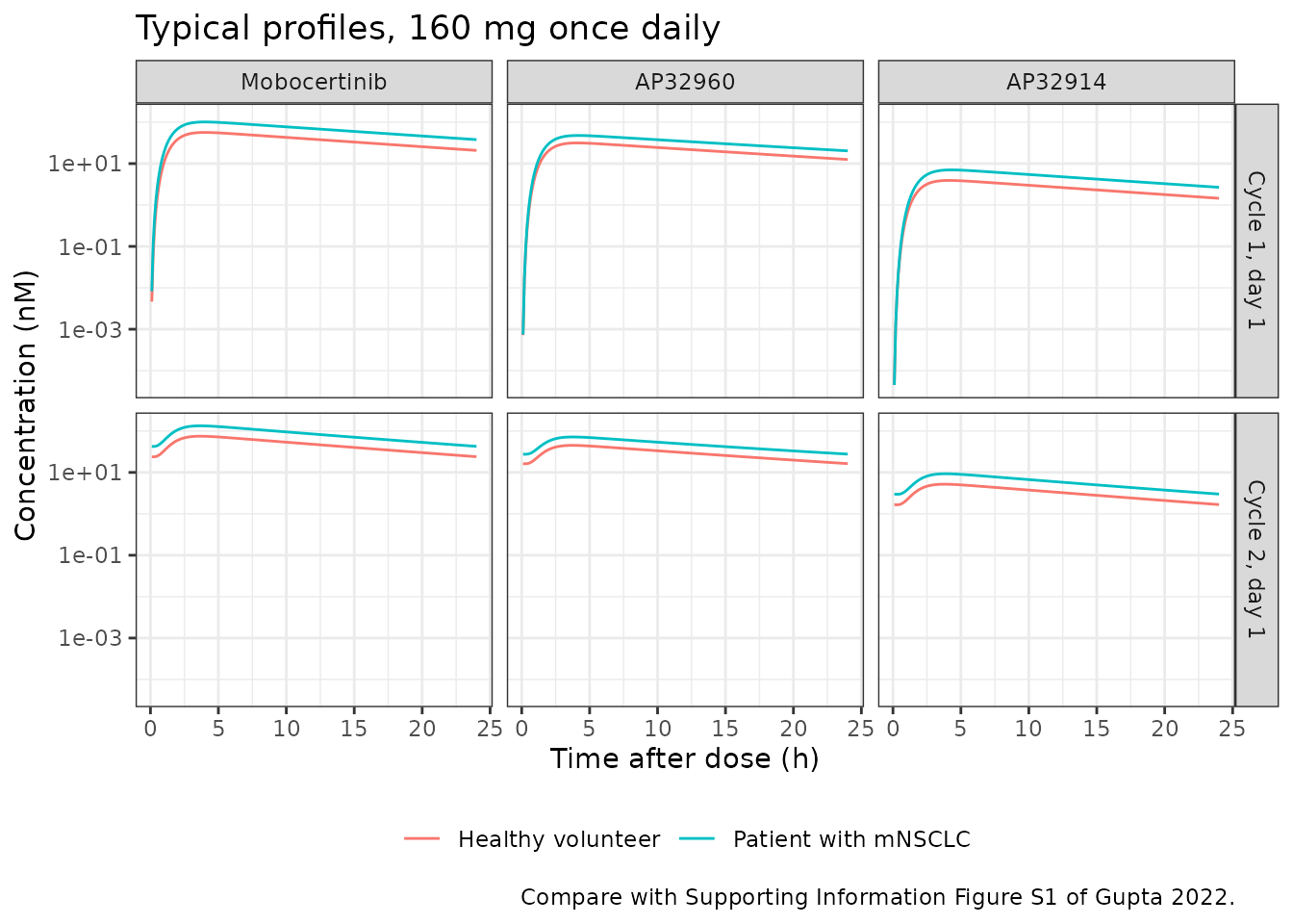
Virtual cohort
Observed data are not public, so the stochastic checks use a virtual cohort. The paper’s covariate analysis simulated every individual in the dataset on continuous 160 mg once-daily dosing and compared the molar-sum AUC0-24h on cycle 2, day 1 between healthy volunteers and patients (Figure 4a). The cohort below does the same with 200 patients and 200 healthy volunteers. Healthy- volunteer status is the only covariate in the model, so no other covariates are drawn.
The studies ran 28-day cycles (Table 1: cycle 1 sampling on days 1, 8, 15 and 22, then cycle 2, day 1), so cycle 2, day 1 is day 29 (672-696 h). Dosing stops after the cycle 2, day 1 dose, and sampling continues for 7 days so that the steady-state half-lives can be estimated by noncompartmental analysis.
set.seed(20220611)
rxode2::rxSetSeed(20220611)

n_per_arm <- 200L
covs <- data.frame(
  id = seq_len(2L * n_per_arm),
  DIS_HEALTHY = rep(c(0L, 1L), each = n_per_arm)
) |>
  dplyr::mutate(
    treatment = ifelse(DIS_HEALTHY == 1L, "Healthy volunteers", "Patients with mNSCLC")
  )
obs_cohort <- sort(unique(c(
  seq(0, 24, by = 0.5), seq(672, 696, by = 0.5), seq(696, 840, by = 4)
)))
events <- make_events(
  ids = covs$id, dose_mg = 160, n_doses = 29L,
  obs_times = obs_cohort, covs = covs
)
stopifnot(!anyDuplicated(events[, c("id", "time", "evid")]))
Simulation
sim <- rxode2::rxSolve(
  mod, events = events, keep = c("treatment", "DIS_HEALTHY"),
  useLinCmt = FALSE
) |>
  as.data.frame() |>
  add_nm()
#> ℹ parameter labels from comments will be replaced by 'label()'
Prediction intervals in patients (Figure 3)
Figure 3 of the paper is a prediction-corrected VPC of the observed data. Without the data, the figure below shows the model’s 5th, 50th and 95th percentiles of mobocertinib and of the molar sum in patients on 160 mg once daily, on cycle 1, day 1 and cycle 2, day 1.
# Model prediction intervals on the time scale of Figure 3 of Gupta 2022.
sim |>
  dplyr::filter(DIS_HEALTHY == 0, time <= 24 | (time >= 672 & time <= 696)) |>
  dplyr::mutate(
    day = ifelse(time <= 24, "Cycle 1, day 1", "Cycle 2, day 1"),
    tad = ifelse(time <= 24, time, time - 672)
  ) |>
  tidyr::pivot_longer(c(Mobocertinib, `Molar sum`), names_to = "analyte", values_to = "conc_nM") |>
  dplyr::group_by(analyte, day, tad) |>
  dplyr::summarise(
    Q05 = quantile(conc_nM, 0.05), Q50 = median(conc_nM), Q95 = quantile(conc_nM, 0.95),
    .groups = "drop"
  ) |>
  dplyr::filter(tad > 0) |>
  ggplot(aes(tad, Q50)) +
  geom_ribbon(aes(ymin = Q05, ymax = Q95), alpha = 0.25) +
  geom_line() +
  facet_grid(analyte ~ day, scales = "free_y") +
  scale_y_log10() +
  labs(
    x = "Time after dose (h)", y = "Concentration (nM)",
    title = "Patients, 160 mg once daily: median and 90% prediction interval",
    caption = "Compare with Figure 3 of Gupta 2022."
  ) +
  theme_bw()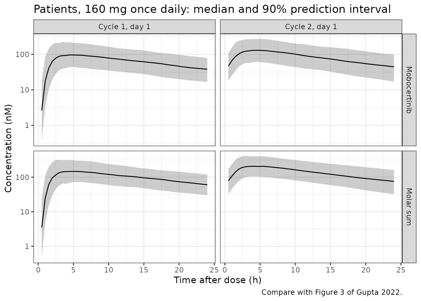
Apparent volume at steady state
The paper reports a geometric mean Vss/F of 3509 L (38% CV) for mobocertinib, derived from the final-model parameters. In the simulated patients, Vss/F is the individual Vc/F plus Vp/F.
vss <- sim |>
  dplyr::distinct(id, DIS_HEALTHY, vc, vp) |>
  dplyr::mutate(vss = vc + vp)
vss_pat <- dplyr::filter(vss, DIS_HEALTHY == 0)
vss_gm <- exp(mean(log(vss_pat$vss)))
vss_cv <- 100 * sqrt(exp(var(log(vss_pat$vss))) - 1)
c(geometric_mean_L = vss_gm, cv_pct = vss_cv)
#> geometric_mean_L           cv_pct
#>        3497.5211          35.0325
stopifnot(abs(vss_gm / 3509 - 1) < 0.10)
The patients’ geometric mean agrees with the published value. Including the healthy volunteers in the analysis proportion (110 of 427) would raise it to about 3950 L, so the published value appears to describe the patients.
PKNCA validation
PKNCA is run once per analyte on the virtual cohort, grouped by treatment. The intervals are the cycle 1, day 1 and cycle 2, day 1 dosing intervals (Cmax, Tmax, AUC0-24h, and a half-life with PKNCA’s automatic point selection within the dosing interval), and the terminal phase from 24 to 168 h after the cycle 2, day 1 dose, which was the last dose.
A second pass estimates the half-life over a fixed window, 24 to 72 h
after the last dose, using every sample in the window (PKNCA
include_half.life). The next section explains why.
PKNCA::PKNCA.options(progress = FALSE)
intervals <- data.frame(
  start = c(0, 672, 696), end = c(24, 696, 840),
  cmax = c(TRUE, TRUE, FALSE), tmax = c(TRUE, TRUE, FALSE),
  auclast = c(TRUE, TRUE, FALSE), half.life = c(FALSE, TRUE, TRUE)
)
intervals_window <- data.frame(start = 696, end = 744, half.life = TRUE)
dose_df <- events |>
  dplyr::filter(evid == 1) |>
  dplyr::select(id, time, amt, treatment)

run_nca <- function(analyte, nca_intervals, window = NULL) {
  conc_df <- sim |>
    dplyr::filter(!is.na(.data[[analyte]])) |>
    dplyr::transmute(id, time, treatment, conc = .data[[analyte]])
  conc_df <- dplyr::bind_rows(
    conc_df,
    conc_df |> dplyr::distinct(id, treatment) |> dplyr::mutate(time = 0, conc = 0)
  ) |>
    dplyr::distinct(id, treatment, time, .keep_all = TRUE) |>
    dplyr::arrange(id, time)
  if (is.null(window)) {
    conc_obj <- PKNCA::PKNCAconc(conc_df, conc ~ time | treatment + id)
  } else {
    conc_df$in_window <- conc_df$time >= window[1] & conc_df$time <= window[2]
    conc_obj <- PKNCA::PKNCAconc(
      conc_df, conc ~ time | treatment + id, include_half.life = "in_window"
    )
  }
  dose_obj <- PKNCA::PKNCAdose(dose_df, amt ~ time | treatment + id)
  res <- PKNCA::pk.nca(PKNCA::PKNCAdata(conc_obj, dose_obj, intervals = nca_intervals))
  as.data.frame(res$result) |>
    dplyr::mutate(analyte = analyte)
}

analytes <- c("Mobocertinib", "AP32960", "AP32914", "Molar sum")
nca <- dplyr::bind_rows(lapply(analytes, run_nca, nca_intervals = intervals)) |>
  dplyr::mutate(
    occasion = dplyr::case_when(
      start == 0 ~ "Cycle 1, day 1",
      start == 672 ~ "Cycle 2, day 1",
      TRUE ~ "Terminal, 24-168 h after the last dose"
    )
  )
nca_window <- dplyr::bind_rows(lapply(
  analytes, run_nca,
  nca_intervals = intervals_window, window = c(696, 744)
)) |>
  dplyr::mutate(occasion = "Fixed window, 24-72 h after the last dose")

nca |>
  dplyr::filter(
    PPTESTCD %in% c("cmax", "tmax", "auclast", "half.life"),
    # tmax is computed internally for the terminal half-life; it is not a
    # result for that interval.
    !(start == 696 & PPTESTCD == "tmax")
  ) |>
  dplyr::group_by(analyte, treatment, occasion, PPTESTCD) |>
  dplyr::summarise(median = signif(median(PPORRES, na.rm = TRUE), 3), .groups = "drop") |>
  tidyr::pivot_wider(names_from = PPTESTCD, values_from = median) |>
  dplyr::rename(
    "Analyte" = analyte, "Treatment" = treatment, "Occasion" = occasion,
    "Cmax (nM)" = cmax, "Tmax (h)" = tmax, "AUC0-24 (nM*h)" = auclast,
    "t1/2 (h)" = half.life
  ) |>
knitr::kable(caption = "Simulated NCA medians, 160 mg once daily.")| Analyte | Treatment | Occasion | AUC0-24 (nM*h) | Cmax (nM) | Tmax (h) | t1/2 (h) |
|---|---|---|---|---|---|---|
| AP32914 | Healthy volunteers | Cycle 1, day 1 | 58.3 | 3.91 | 4.0 | NA |
| AP32914 | Healthy volunteers | Cycle 2, day 1 | 75.8 | 5.21 | 4.0 | 12.1 |
| AP32914 | Healthy volunteers | Terminal, 24-168 h after the last dose | NA | NA | NA | 69.3 |
| AP32914 | Patients with mNSCLC | Cycle 1, day 1 | 106.0 | 6.86 | 4.5 | NA |
| AP32914 | Patients with mNSCLC | Cycle 2, day 1 | 141.0 | 9.54 | 4.0 | 12.3 |
| AP32914 | Patients with mNSCLC | Terminal, 24-168 h after the last dose | NA | NA | NA | 75.1 |
| AP32960 | Healthy volunteers | Cycle 1, day 1 | 494.0 | 31.50 | 4.0 | NA |
| AP32960 | Healthy volunteers | Cycle 2, day 1 | 726.0 | 46.50 | 3.5 | 14.0 |
| AP32960 | Healthy volunteers | Terminal, 24-168 h after the last dose | NA | NA | NA | 53.6 |
| AP32960 | Patients with mNSCLC | Cycle 1, day 1 | 741.0 | 46.30 | 4.0 | NA |
| AP32960 | Patients with mNSCLC | Cycle 2, day 1 | 1170.0 | 73.10 | 3.5 | 15.7 |
| AP32960 | Patients with mNSCLC | Terminal, 24-168 h after the last dose | NA | NA | NA | 59.9 |
| Mobocertinib | Healthy volunteers | Cycle 1, day 1 | 853.0 | 56.40 | 4.0 | NA |
| Mobocertinib | Healthy volunteers | Cycle 2, day 1 | 1120.0 | 77.00 | 3.5 | 12.1 |
| Mobocertinib | Healthy volunteers | Terminal, 24-168 h after the last dose | NA | NA | NA | 69.4 |
| Mobocertinib | Patients with mNSCLC | Cycle 1, day 1 | 1550.0 | 103.00 | 4.0 | NA |
| Mobocertinib | Patients with mNSCLC | Cycle 2, day 1 | 2020.0 | 134.00 | 3.5 | 12.3 |
| Mobocertinib | Patients with mNSCLC | Terminal, 24-168 h after the last dose | NA | NA | NA | 75.1 |
| Molar sum | Healthy volunteers | Cycle 1, day 1 | 1420.0 | 90.20 | 4.0 | NA |
| Molar sum | Healthy volunteers | Cycle 2, day 1 | 1940.0 | 128.00 | 3.5 | 12.8 |
| Molar sum | Healthy volunteers | Terminal, 24-168 h after the last dose | NA | NA | NA | 60.4 |
| Molar sum | Patients with mNSCLC | Cycle 1, day 1 | 2370.0 | 155.00 | 4.0 | NA |
| Molar sum | Patients with mNSCLC | Cycle 2, day 1 | 3270.0 | 214.00 | 3.5 | 13.3 |
| Molar sum | Patients with mNSCLC | Terminal, 24-168 h after the last dose | NA | NA | NA | 67.6 |
Comparison against published steady-state half-lives
The paper reports geometric mean (CV%) steady-state elimination half-lives in patients of 18 h (21%) for mobocertinib, 24 h (20%) for AP32960 and 18 h (21%) for AP32914, from NCA of the simulated profiles. It does not say which samples the half-life was fitted to.
That matters here, because mobocertinib and AP32960 have a slow distribution phase. The mobocertinib peripheral rate constant is Q/Vp = 11.7 / 1110 = 0.0105 /h, a half-life of 66 h. So the apparent half-life rises steadily the later after the dose it is measured: about 12 h within the dosing interval and about 75 h in the terminal phase. AP32914 is formed from mobocertinib and follows its decline. The table below shows all three estimates. The published values lie between the in-interval and terminal estimates. The fixed 24-72 h window reproduces them, which is consistent with a fit to samples one to three days after the last dose, but that window is the maintainers’ reconstruction, not something the paper states.
hl_all <- dplyr::bind_rows(nca, nca_window) |>
  dplyr::filter(
    PPTESTCD == "half.life", treatment == "Patients with mNSCLC",
    analyte != "Molar sum", !is.na(PPORRES)
  ) |>
  dplyr::group_by(analyte, occasion) |>
  dplyr::summarise(
    cv = 100 * sqrt(exp(var(log(PPORRES))) - 1),
    gm = exp(mean(log(PPORRES))),
    .groups = "drop"
  )
hl_all |>
  dplyr::mutate(gm = signif(gm, 3), cv = round(cv)) |>
  dplyr::rename(
    "Analyte" = analyte, "Half-life estimate" = occasion,
    "Geometric mean (h)" = gm, "CV (%)" = cv
  ) |>
knitr::kable(caption = "Simulated steady-state half-lives in patients by NCA window.")| Analyte | Half-life estimate | CV (%) | Geometric mean (h) |
|---|---|---|---|
| AP32914 | Cycle 2, day 1 | 26 | 12.5 |
| AP32914 | Fixed window, 24-72 h after the last dose | 19 | 19.3 |
| AP32914 | Terminal, 24-168 h after the last dose | 9 | 74.7 |
| AP32960 | Cycle 2, day 1 | 25 | 16.1 |
| AP32960 | Fixed window, 24-72 h after the last dose | 20 | 25.3 |
| AP32960 | Terminal, 24-168 h after the last dose | 10 | 59.8 |
| Mobocertinib | Cycle 2, day 1 | 26 | 12.5 |
| Mobocertinib | Fixed window, 24-72 h after the last dose | 20 | 19.4 |
| Mobocertinib | Terminal, 24-168 h after the last dose | 9 | 74.7 |
hl_sim <- hl_all |>
  dplyr::filter(occasion == "Fixed window, 24-72 h after the last dose") |>
  dplyr::transmute(analyte, PPTESTCD = "half.life", PPORRES = gm, cv)
hl_pub <- data.frame(
  analyte = c("Mobocertinib", "AP32960", "AP32914"),
  half.life = c(18, 24, 18),
  cv_pub = c(21, 20, 21)
)
cmp <- nlmixr2lib::ncaComparisonTable(
  simulated = dplyr::select(hl_sim, analyte, PPTESTCD, PPORRES),
  reference = dplyr::select(hl_pub, analyte, half.life),
  by = "analyte",
  tolerance_pct = 20
)
knitr::kable(
  cmp,
  caption = paste(
    "Geometric mean steady-state half-life in patients (fixed 24-72 h window)",
    "versus Gupta 2022 (Results, 'Model-based simulations').",
    "* differs from the published value by more than 20%."
  )
)| NCA parameter | analyte | Reference | Simulated | % diff |
|---|---|---|---|---|
| t½ | Mobocertinib | 18 | 19.4 | +7.9% |
| t½ | AP32960 | 24 | 25.3 | +5.3% |
| t½ | AP32914 | 18 | 19.3 | +7.3% |
The gate checks the fixed-window values against the published ones. It also checks a quantity that does not depend on the window: the ratio of the AP32960 and mobocertinib half-lives, published as 24 / 18 = 1.33. Across the in-interval and fixed-window estimates the simulated ratio stays near 1.3, so a mis-transcribed metabolite clearance or volume would show up here whichever window the paper used.
The fixed window also reproduces the published between-subject CVs (about 20%, against 20-21%), whereas the in-interval estimates vary more (about 26%) and the terminal estimates much less (about 10%). That supports the window as the one the paper used.
hl_gate <- dplyr::inner_join(hl_sim, hl_pub, by = "analyte") |>
  dplyr::mutate(pct = 100 * (PPORRES - half.life) / half.life)
hl_ratio <- hl_all |>
  dplyr::filter(occasion != "Terminal, 24-168 h after the last dose") |>
  dplyr::group_by(occasion) |>
  dplyr::summarise(
    ratio = gm[analyte == "AP32960"] / gm[analyte == "Mobocertinib"],
    .groups = "drop"
  )
hl_ratio
#> # A tibble: 2 × 2
#>   occasion                                  ratio
#>   <chr>                                     <dbl>
#> 1 Cycle 2, day 1                             1.28
#> 2 Fixed window, 24-72 h after the last dose  1.30
stopifnot(
  nrow(hl_gate) == 3L,
  # Geometric means of 200 subjects; Monte Carlo error is about 2%.
  all(abs(hl_gate$pct) < 15),
  nrow(hl_ratio) == 2L,
  all(abs(hl_ratio$ratio / (24 / 18) - 1) < 0.15)
)
Healthy volunteers versus patients (Figure 4a)
Figure 4a gives the mean molar-sum AUC0-24h on cycle 2, day 1 as 43.1% lower in healthy volunteers than in patients with mNSCLC.
auc_c2 <- nca |>
  dplyr::filter(analyte == "Molar sum", PPTESTCD == "auclast", occasion == "Cycle 2, day 1")
auc_means <- auc_c2 |>
  dplyr::group_by(treatment) |>
  dplyr::summarise(mean_auc = mean(PPORRES), .groups = "drop")
pct_hv <- 100 * (auc_means$mean_auc[auc_means$treatment == "Healthy volunteers"] /
  auc_means$mean_auc[auc_means$treatment == "Patients with mNSCLC"] - 1)
pct_hv
#> [1] -42.05929

# Replicates Figure 4a of Gupta 2022.
ggplot(auc_c2, aes(treatment, PPORRES / 1000)) +
  geom_boxplot(outlier.shape = NA) +
  geom_jitter(width = 0.15, alpha = 0.3, size = 0.8) +
  geom_point(
    data = auc_means, aes(treatment, mean_auc / 1000), colour = "red", size = 3
  ) +
  labs(
    x = NULL, y = "Molar-sum AUC0-24h, cycle 2 day 1 (uM*h)",
    title = sprintf("Healthy volunteers %.1f%% vs patients (published -43.1%%)", pct_hv),
    caption = "Replicates Figure 4a of Gupta 2022. Red points are means."
  ) +
  theme_bw()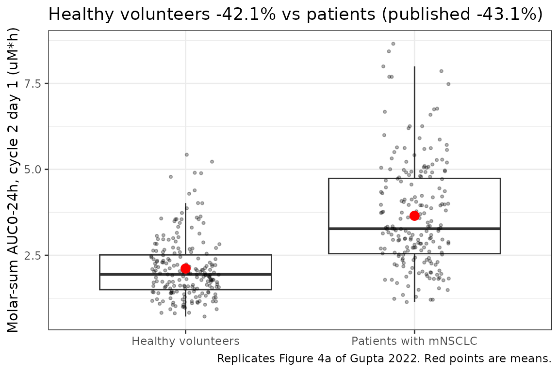
# Each arm mean has a Monte Carlo error of about 3.5% with 200 subjects, so
# the difference is gated with about 7 percentage points of room either side.
stopifnot(pct_hv > -50, pct_hv < -36)
Figure 4b also reports that the 5th and 95th percentiles of the individual molar-sum AUC0-24h across the patients were -47% and +191% relative to the median. Those percentiles came from individual (post hoc) predictions; the simulated patients give the following, shown without a gate. The lower percentile agrees. The upper one is narrower in the simulation (about +100%). The post hoc values reflect each patient’s estimated parameters, which this simulation from the population distribution cannot reproduce, and the tail of a skewed distribution is sensitive to a few patients with very low clearance.
Assumptions and deviations
- Molecular weight. The paper fits the model in molar units and gives the EC50 in nM, but does not print a molecular weight. Doses are converted with the mobocertinib free-base molecular weight of 585.7 g/mol (PubChem CID 118607832), taking the labelled dose as free-base mobocertinib. The metabolite molecular weights are not reported, so the metabolites are shown in nM only.
-
Fixed metabolite fractions. The 62% and 8%
fractions are hardcoded in the control stream
$PKand taken from earlier clinical data (Methods); they are encoded withfixed(). Because the formation flux is in moles, they are molar fractions. - Transit chain. The control stream has a depot and three transit compartments, each emptied at rate ka, so the dose passes through four first-order steps before reaching the central compartment. This matches Figure 1 (“Ka = Ktr”).
-
Emax on the log scale. The authors estimated Emax
untransformed (
EMAX = THETA(21)). It is held here aslemax = log(0.781), which gives the same value. Its bootstrap 95% CI (0.301-417) and that of EC50 (16.9-225,000 nM) are very wide, so the induction parameters are individually poorly determined, although their combined effect is constrained by the data. - Days of the simulated checks. Steady state for the typical-value Cmax is taken at the 60th daily dose, after induction is complete. Cycle 2, day 1 is taken as day 29 from the 28-day cycle schedule in Table 1.
- Half-life window. The paper does not say which samples its steady-state half-lives were fitted to. Because of the slow distribution phase the answer depends strongly on the window (about 12 h within the dosing interval, about 75 h in the terminal phase). The comparison uses a 24-72 h window after the cycle 2, day 1 dose, which reproduces the published values; the window was chosen by the maintainers for that reason, and the in-interval and terminal values are shown alongside it.
- Healthy-volunteer arm. As in the paper’s Figure 4a simulation, healthy volunteers are simulated on continuous once-daily dosing, although in the studies they received single doses only. The healthy-volunteer effects were estimated from single-dose data, and the paper notes that the lack of multiple-dose data in healthy volunteers may be part of the difference.
-
Screened covariates. Age, body weight, sex, race,
albumin, ALT, AST, total bilirubin, eGFR, smoking status and drug
product were screened and not retained. They are listed in the model’s
covariatesDataExcluded. - Bioequivalence refits not encoded. The paper also refitted adapted versions of the final model with drug-product effects on ka and F, to assess capsule B versus capsule A and capsule C versus capsules A/B (Supporting Information Tables S2 and S4). Both refits concluded that the capsules are bioequivalent. They are secondary analyses rather than the final model, and are not packaged.
-
Residual error. The model was fitted with
log-transform-both-sides and an additive error on the log scale, with
independent errors for the three analytes. That is the
lnorm()error model here. Concentrations below the lower limit of quantification were handled by a modified M6 method in the fit; nothing in this model depends on that. - No erratum or correction notice for this article is linked in Europe PMC (PMID 35316867) as of 2026-10-01.