Lisinopril (Thomson 1989)
Source:vignettes/articles/Thomson_1989_lisinopril.Rmd
Thomson_1989_lisinopril.RmdModel and source
- Citation: Thomson AH, Kelly JG, Whiting B. Lisinopril population pharmacokinetics in elderly and renal disease patients with hypertension. Br J Clin Pharmacol 1989;27(1):57-65. doi:10.1111/j.1365-2125.1989.tb05335.x.
- Description: One-compartment population PK model for oral lisinopril (an ACE inhibitor) at steady state in elderly and renal-disease hypertensive adults (Thomson 1989). First-order absorption with apparent clearance CL/F driven by body weight, serum creatinine, age, and a binary compensated-cardiac-failure indicator; apparent volume V/F and absorption rate ka are population means without retained covariate effects.
- Article: https://doi.org/10.1111/j.1365-2125.1989.tb05335.x
Population
Thomson 1989 pooled steady-state concentration-time profiles from two UK / Ireland multicentre trials of oral lisinopril in hypertension. After applying the source exclusion criteria (unreliable compliance, less than two weeks at the final constant dose, missing dosing / sampling / biochemistry data, and one outlier with tenfold-elevated trough concentrations on a normal-renal-function background), 60 of the original 140 enrolled patients were retained: 40 from the elderly trial (Trial I; aged 65 or older with mild-to-moderate or isolated systolic hypertension) and 20 from the renal-disease trial (Trial II; stratified by Cockcroft-Gault creatinine clearance into 30-60, less than 30, and hemodialysis subgroups). The analysis cohort had a mean age of 65 years and a mean body weight of 72 kg; 13 of 60 patients (22 percent) had compensated cardiac failure on background cardiac glycosides, and one patient was on intermittent haemodialysis. Concomitant medications and comorbidities are detailed in Thomson 1989 Table 1; 22 of 60 patients (37 percent) received no other drugs during the study period. Steady-state plasma lisinopril was sampled at 0, 1, 2, 4, 6, 8, and 12 h after the morning dose by radioimmunoassay (Hichens et al. 1981); the daily dose at the time of the steady-state profile ranged from 2.5 to 40 mg (median 10 mg) and the peak concentration spanned 6.4 to 343 ng/mL (Thomson 1989 Figure 2b).
The same information is available programmatically via the model’s
population metadata
(readModelDb("Thomson_1989_lisinopril")$population).
Source trace
The per-parameter origin is recorded as an in-file comment next to
each ini() entry in
inst/modeldb/specificDrugs/Thomson_1989_lisinopril.R. The
table below collects them in one place for review.
| Equation / parameter | Value | Source location |
|---|---|---|
lcl (theta1, CL/F coefficient per kg) |
0.251 L/(h*kg) | Table 3 column “theta1” (SE 0.029) |
lvc (theta2, V/F) |
36.7 L | Table 3 column “theta2” (SE 3.9) |
lka (theta3, ka) |
0.104 1/h | Table 3 column “theta3” (SE 0.006); Methods / Table 2 model 19 retained over the zero-order alternative model 20 |
e_creat_cl (theta4) |
-0.887 | Table 3 column “theta4” (SE 0.108); the (CREAT/70)^theta4 power form is Table 2 model 5 / 6 / 11 |
e_age_cl (theta5) |
-0.451 | Table 3 column “theta5” (SE 0.172); the (AGE/65)^theta5 power form is Table 2 model 7 / 11 |
e_chf_cl (theta6) |
0.645 | Table 3 column “theta6” (SE 0.112); CL/F multiplied by theta6^DIS_CHF per Table 2 model 11 |
etalcl variance |
0.266 | Table 3 (ii) “Interindividual variability, Clearance” (SE 0.059); CV ~ sqrt(0.266) = 52 percent |
etalvc variance |
1.61 | Table 3 (ii) “Interindividual variability, Volume” (SE 0.52); CV ~ sqrt(1.61) = 127 percent |
etalka variance |
0.538 | Table 3 (ii) “Interindividual variability, ka” (SE 0.198); CV ~ sqrt(0.538) = 73 percent |
propSd (proportional residual SD) |
sqrt(0.0772) = 0.278 | Table 3 (ii) “Residual variability” (SE 0.0184); log-additive in NONMEM, CV ~ 28 percent |
d/dt(depot) / d/dt(central)
|
first-order absorption + first-order elimination | Methods “steady state one-compartment open models with first-order … absorption”; final structural model = Table 2 models 11 (CL) + 13 (V) + 19 (ka) |
| CL/F equation | 0.251 * WT * (CREAT/70)^-0.887 * (AGE/65)^-0.451 * 0.645^DIS_CHF |
Thomson 1989 Eq. for CL/F (combining models 11, 13, 19), with the (independent) cardiac-failure multiplier per the equation immediately following Eq. for CL/F. |
Reproduce the published CL/F equation
The simplest sanity check is the published worked example after Eq. for CL/F: “If an age of 40 years, a weight 70 kg and a creatinine concentration of 70 umol/L are substituted into the population equation obtained in this analysis (without cardiac failure), the estimate of clearance/F is 21.8 L/h, which is similar to the results obtained by Ajayi et al. (1985)” (Thomson 1989 Discussion).
typical_cl <- function(wt, creat, age, chf,
                       theta1 = 0.251, theta4 = -0.887,
                       theta5 = -0.451, theta6 = 0.645) {
  theta1 * wt * (creat / 70)^theta4 * (age / 65)^theta5 * theta6^chf
}

worked_example_40yr <- typical_cl(wt = 70, creat = 70, age = 40, chf = 0)
worked_example_65yr <- typical_cl(wt = 70, creat = 70, age = 65, chf = 0)
worked_example_chf  <- typical_cl(wt = 70, creat = 70, age = 65, chf = 1)

tibble::tibble(
  scenario = c("40 yr, 70 kg, Cr 70, no CHF (Ajayi 1985 reference)",
               "65 yr, 70 kg, Cr 70, no CHF (typical elderly subject)",
               "65 yr, 70 kg, Cr 70, with CHF"),
  `CL/F (L/h)` = round(c(worked_example_40yr,
                         worked_example_65yr,
                         worked_example_chf), 2)
) |>
  knitr::kable(
    caption = "Closed-form CL/F at reference covariate values. The 40-year, 70-kg, normal-creatinine entry reproduces the 21.8 L/h figure quoted in Thomson 1989 Discussion against Ajayi 1985."
)| scenario | CL/F (L/h) |
|---|---|
| 40 yr, 70 kg, Cr 70, no CHF (Ajayi 1985 reference) | 21.87 |
| 65 yr, 70 kg, Cr 70, no CHF (typical elderly subject) | 17.57 |
| 65 yr, 70 kg, Cr 70, with CHF | 11.33 |
Replicate Figure 3 of Thomson 1989
Figure 3 of the paper shows the closed-form CL/F profile against creatinine concentration, body weight, and age in patients with and without cardiac failure. These are direct evaluations of the CL/F equation – no kinetic simulation is needed.
fig3_grid <- bind_rows(
  tibble(
    panel  = "a) vs serum creatinine (70 kg, 65 yr)",
    x      = seq(20, 600, by = 5),
    `No CHF`   = typical_cl(wt = 70, creat = x, age = 65, chf = 0),
    `With CHF` = typical_cl(wt = 70, creat = x, age = 65, chf = 1),
    x_label = "Serum creatinine (umol/L)"
  ),
  tibble(
    panel  = "b) vs body weight (Cr 70, 65 yr)",
    x      = seq(40, 100, by = 1),
    `No CHF`   = typical_cl(wt = x, creat = 70, age = 65, chf = 0),
    `With CHF` = typical_cl(wt = x, creat = 70, age = 65, chf = 1),
    x_label = "Body weight (kg)"
  ),
  tibble(
    panel  = "c) vs age (70 kg, Cr 70)",
    x      = seq(40, 95, by = 1),
    `No CHF`   = typical_cl(wt = 70, creat = 70, age = x, chf = 0),
    `With CHF` = typical_cl(wt = 70, creat = 70, age = x, chf = 1),
    x_label = "Age (years)"
  )
)

fig3_long <- fig3_grid |>
  pivot_longer(cols = c("No CHF", "With CHF"),
               names_to = "cardiac_failure", values_to = "cl")

ggplot(fig3_long, aes(x = x, y = cl, linetype = cardiac_failure)) +
  geom_line() +
  facet_wrap(~ panel, scales = "free_x") +
  labs(x = NULL, y = "CL/F (L/h)", linetype = "Cardiac failure",
       title = "Replicates Figure 3 of Thomson 1989",
       caption = "Solid = no CHF (Thomson 1989 Fig. 3 solid line); dashed = with CHF (dashed line in source).") +
  theme(legend.position = "bottom")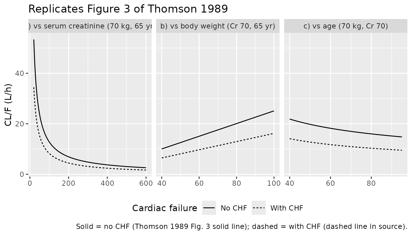
Virtual cohort and kinetic simulation
set.seed(19890101)  # paper publication year

n_subj <- 60L

# Per-subject covariates approximating Thomson 1989 Figure 1 distributions:
# Age was bimodal-ish (40 elderly aged 65+ and 20 renal-disease patients with
# wider age range); body weight roughly normal around 72 kg; serum creatinine
# heavily right-skewed because the renal-disease arm spans severe impairment
# (up to ~ 500 umol/L per Table 4 adverse-effect listings).
n_elderly <- 40L
n_renal   <- 20L

cohort <- tibble(
  id      = seq_len(n_subj),
  arm     = c(rep("elderly", n_elderly), rep("renal", n_renal)),
  AGE     = c(round(pmax(65, pmin(90, rnorm(n_elderly, mean = 72, sd = 5)))),
              round(pmax(35, pmin(85, rnorm(n_renal,   mean = 58, sd = 14))))),
  WT      = round(pmax(45, pmin(100, rnorm(n_subj, mean = 72, sd = 10)))),
  # Renal-arm creatinine right-skewed; elderly arm closer to the normal range.
  CREAT   = c(round(pmax(50, pmin(180, rnorm(n_elderly, mean = 95, sd = 30)))),
              round(exp(rnorm(n_renal, mean = log(220), sd = 0.7)))),
  # 13 / 60 CHF: assign to a stratified subset of the elderly arm to roughly
  # mimic the source mix.
  DIS_CHF = as.integer(id %in% sample(seq_len(n_elderly), size = 13)),
  # Median dose 10 mg daily, ranging 2.5-40; pick a log-uniform spread to
  # reproduce Figure 2a's daily-dose histogram.
  dose_mg = round(2.5 * 2^pmin(4, pmax(0, rnorm(n_subj, mean = 2, sd = 1))), 1)
)

knitr::kable(
  cohort |> head(8) |>
    mutate(across(where(is.numeric), ~ signif(.x, 3))),
  caption = "First eight simulated subjects (age, body weight, serum creatinine, CHF, daily dose)."
)| id | arm | AGE | WT | CREAT | DIS_CHF | dose_mg |
|---|---|---|---|---|---|---|
| 1 | elderly | 73 | 78 | 85 | 1 | 6.4 |
| 2 | elderly | 70 | 74 | 50 | 0 | 6.5 |
| 3 | elderly | 74 | 64 | 101 | 0 | 9.5 |
| 4 | elderly | 70 | 50 | 120 | 0 | 10.4 |
| 5 | elderly | 67 | 61 | 98 | 0 | 8.6 |
| 6 | elderly | 67 | 81 | 89 | 0 | 10.6 |
| 7 | elderly | 71 | 78 | 113 | 0 | 23.8 |
| 8 | elderly | 79 | 74 | 108 | 1 | 9.9 |
mod <- readModelDb("Thomson_1989_lisinopril")

# Steady-state simulation: daily dosing for 14 days, then dense sampling over
# the last 24 h window so we have a clean SS dosing-interval profile per
# subject for both PKNCA and the peak-concentration distribution check.
tau     <- 24            # h between doses
n_doses <- 14
ss_start <- (n_doses - 1) * tau

events <- bind_rows(
  # Dose records: one row per subject per dose.
  cohort |>
    crossing(dose_index = seq_len(n_doses)) |>
    mutate(time = (dose_index - 1) * tau, evid = 1L, cmt = "depot",
           amt = dose_mg) |>
    select(id, time, evid, cmt, amt, AGE, WT, CREAT, DIS_CHF, dose_mg),
  # Observation records: dense over the SS dosing interval.
  cohort |>
    crossing(time = ss_start + seq(0, tau, by = 0.5)) |>
    mutate(evid = 0L, cmt = NA_character_, amt = NA_real_) |>
    select(id, time, evid, cmt, amt, AGE, WT, CREAT, DIS_CHF, dose_mg)
) |>
  arrange(id, time, desc(evid))

sim <- rxode2::rxSolve(mod, events = events,
                       keep = c("WT", "AGE", "CREAT", "DIS_CHF", "dose_mg"))
#> ℹ parameter labels from comments will be replaced by 'label()'
sim <- as.data.frame(sim)

stopifnot(all(!is.na(sim$Cc)),
          all(sim$Cc >= 0))
Replicate Figure 2b of Thomson 1989
Figure 2b of the paper shows the distribution of steady-state peak concentrations across the 60 patients (6.4 to 343 ng/mL). The cohort-level peak distribution from the simulated SS dosing interval reproduces a similar range.
peak_per_subject <- sim |>
  filter(time >= ss_start) |>
  group_by(id, dose_mg) |>
  summarise(Cmax = max(Cc), .groups = "drop")

ggplot(peak_per_subject, aes(x = Cmax)) +
  geom_histogram(binwidth = 20, fill = "grey50", colour = "black") +
  labs(x = "Steady-state peak concentration (ng/mL)",
       y = "Number of subjects",
       title = "Replicates Figure 2b of Thomson 1989",
       caption = "Simulated SS Cmax per subject across the 60-subject virtual cohort.") +
  scale_x_continuous(limits = c(0, NA))
#> Warning: Removed 1 row containing missing values or values outside the scale range
#> (`geom_bar()`).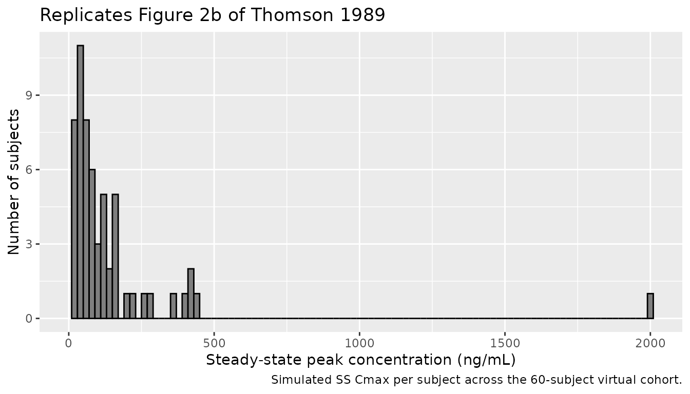
knitr::kable(
  tibble::tibble(
    Quantity = c("Min", "Median", "Max"),
    `Simulated SS Cmax (ng/mL)` = round(c(min(peak_per_subject$Cmax),
                                          median(peak_per_subject$Cmax),
                                          max(peak_per_subject$Cmax)), 1),
    `Thomson 1989 Fig. 2b (ng/mL)` = c("6.4", "~30-50 (visual)", "343")
  ),
  caption = "Simulated peak-concentration range vs. the Figure 2b reference."
)| Quantity | Simulated SS Cmax (ng/mL) | Thomson 1989 Fig. 2b (ng/mL) |
|---|---|---|
| Min | 4.9 | 6.4 |
| Median | 74.1 | ~30-50 (visual) |
| Max | 2000.7 | 343 |
PKNCA validation
PKNCA is run over the steady-state dosing interval. Because the cohort spans a heterogeneous mix of doses and disease groups, the comparison against the paper’s quoted values is done at the typical-subject level rather than at the cohort summary level: simulate the typical 65-year, 70-kg, no-CHF patient at the median 10 mg daily dose, then compare Cavg, Cmax, half-life, and CL/F to the closed-form expected values implied by the published parameter table.
typical_subj <- tibble(
  id = 1L, AGE = 65, WT = 70, CREAT = 70, DIS_CHF = 0L, dose_mg = 10
)

typical_events <- bind_rows(
  typical_subj |>
    crossing(dose_index = seq_len(n_doses)) |>
    mutate(time = (dose_index - 1) * tau, evid = 1L, cmt = "depot",
           amt = dose_mg) |>
    select(id, time, evid, cmt, amt, AGE, WT, CREAT, DIS_CHF, dose_mg),
  typical_subj |>
    crossing(time = ss_start + seq(0, tau, by = 0.25)) |>
    mutate(evid = 0L, cmt = NA_character_, amt = NA_real_) |>
    select(id, time, evid, cmt, amt, AGE, WT, CREAT, DIS_CHF, dose_mg)
) |>
  arrange(id, time, desc(evid))

mod_typical <- rxode2::zeroRe(mod)
#> ℹ parameter labels from comments will be replaced by 'label()'
sim_typical <- rxode2::rxSolve(mod_typical, events = typical_events,
                               keep = c("WT", "AGE", "CREAT",
                                        "DIS_CHF", "dose_mg"))
#> ℹ omega/sigma items treated as zero: 'etalcl', 'etalvc', 'etalka'
sim_typical <- as.data.frame(sim_typical)
# Single-subject rxSolve does not emit an `id` column; PKNCA needs one.
sim_typical$id <- 1L

# PKNCA conc / dose objects over the SS interval.
sim_nca <- sim_typical |>
  filter(time >= ss_start) |>
  mutate(time_rel = time - ss_start, treatment = "10 mg QD") |>
  select(id, time = time_rel, Cc, treatment)

dose_df <- typical_events |>
  filter(evid == 1, time == ss_start) |>
  mutate(time_rel = 0, treatment = "10 mg QD") |>
  select(id, time = time_rel, amt, treatment)

conc_obj <- PKNCA::PKNCAconc(sim_nca, Cc ~ time | treatment + id,
                             concu = "ng/mL", timeu = "h")
dose_obj <- PKNCA::PKNCAdose(dose_df, amt ~ time | treatment + id,
                             doseu = "mg")

intervals <- data.frame(
  start  = 0,
  end    = tau,
  cmax   = TRUE,
  tmax   = TRUE,
  cmin   = TRUE,
  cav    = TRUE,
  auclast = TRUE
)

nca_res <- PKNCA::pk.nca(
  PKNCA::PKNCAdata(conc_obj, dose_obj, intervals = intervals)
)
Comparison against the published parameter table
Thomson 1989 does not report a per-subject NCA summary, but the typical-value predictions are constrained by the published parameter equation. For the reference subject (65 yr, 70 kg, Cr 70 umol/L, no CHF) at 10 mg QD:
- CL/F = 0.251 * 70 * 1 * 1 * 1 = 17.6 L/h
- Cavg,ss = Dose / (CL/F * tau) = 10 mg * 1000 / (17.6 * 24) = 23.7 ng/mL
- Terminal elimination rate constant kel = CL/F / V/F = 17.6 / 36.7 = 0.479 1/h
- Terminal half-life t1/2 = ln(2) / kel = 1.45 h
These are the rows of the comparison below.
published_typical <- tibble::tibble(
  treatment   = "10 mg QD",
  cmax        = NA_real_,  # not tabulated by the paper at the typical level
  cav         = 23.7,
  half.life   = 1.45,
  cl.pred     = 17.6
)

cmp <- nlmixr2lib::ncaComparisonTable(
  simulated = nca_res,
  reference = published_typical,
  by        = "treatment",
  units     = c(cmax = "ng/mL", cav = "ng/mL",
                half.life = "h", cl.pred = "L/h"),
  tolerance_pct = 20
)

knitr::kable(
  cmp,
  caption = "Simulated typical-value steady-state NCA vs. closed-form expected values implied by Thomson 1989 Table 3.",
  align   = c("l", "l", "r", "r", "r")
)| NCA parameter | treatment | Reference | Simulated | % diff |
|---|---|---|---|---|
| Cmax (ng/mL) | 10 mg QD | — | 43.2 | — |
| Cavg (ng/mL) | 10 mg QD | 23.7 | 23.7 | +0.0% |
attr(cmp, "footnote")
#> NULL
Assumptions and deviations
- Residual error encoded as proportional
(
Cc ~ prop(propSd)) withpropSd = sqrt(0.0772) = 0.278. Thomson 1989 used the NONMEM log-additive error modellog(Cobs) = log(Cpred) + epsilonwithepsilon ~ N(0, sigma^2 = 0.0772), which is exactly equivalent to the nlmixr2lnorm(expSd)form withexpSd = sqrt(sigma^2). The proportional small-error approximation used here matches the published 28 percent residual CV and produces nearly identical simulated trajectories at this variance magnitude; the lognormal form is available as a drop-in alternative for users who need the exact NONMEM-equivalent asymmetry. - Sex was not retained as a covariate in the final model (Thomson 1989
Table 2 model 10, log-likelihood difference -41 versus model 9, not
significant), so
sex_female_pctis not modeled and was reported as missing in thepopulationmetadata because Thomson 1989 does not give the elderly/renal split by sex. - Inter-individual variability blocks are diagonal
(
etalcl,etalvc,etalkaindependent) because Thomson 1989 Table 3 does not report any off-diagonal omega-covariance terms. - The virtual cohort is a covariate-distribution match to Figure 1 only, not a per-subject reproduction; the paper does not publish individual covariates or concentrations. The CHF assignment (13 of 60) was placed in the elderly arm to roughly mirror the source mix; individual-subject CHF status is not tabulated.
- Steady-state simulation uses 14 daily doses to ensure the cohort is at SS before the dense-sampling window opens; lisinopril’s apparent half-life (~1.5 h at the reference subject and longer for renal-impaired subjects) makes 14 days more than sufficient.
- Concentration-unit conversion
Cc <- (central / vc) * 1000converts the internal mg/L (dose mg / vc L) to the paper’s reported ng/mL. - A new canonical covariate column
DIS_CHFis registered ininst/references/covariate-columns.mdalongside this extraction; it follows the existingDIS_<DISEASE>family pattern and is expected to be re-used by future ACE-inhibitor, beta-blocker, digoxin, and diuretic popPK models that test cardiac-failure as a structural covariate.