Model and source
- Citation: Ku LC, Hornik CP, Beechinor RJ, Chamberlain JM, Guptill JT, Harper B, Capparelli EV, Martz K, Anand R, Cohen-Wolkowiez M, Gonzalez D, on behalf of the Best Pharmaceuticals for Children Act - Pediatric Trials Network Steering Committee. Population Pharmacokinetics and Exploratory Exposure-Response Relationships of Diazepam in Children Treated for Status Epilepticus. CPT Pharmacometrics Syst Pharmacol. 2018;7(11):718-727. doi:10.1002/psp4.12349.
- Description: Two-compartment population PK model for intravenous diazepam in children aged 3 months to 18 years treated for status epilepticus. Clearance, central volume, inter-compartmental clearance, and peripheral volume scale allometrically with total body weight referenced to a 70 kg adult (fixed exponents 0.75 on CL and Q; 1 on V1 and V2). IIV is estimated on CL and V1 only; IIV on Q and V2 was held fixed at 0 in the final model to avoid >50% shrinkage. Proportional residual error.
- Article: https://doi.org/10.1002/psp4.12349 (open access; Wiley)
Ku 2018 describes a two-compartment population PK model of intravenous diazepam in 87 children (3 months to 18 years) treated for status epilepticus, leveraging the PK substudy of the Chamberlain 2014 JAMA trial (NCT00621478) comparing IV diazepam to IV lorazepam. The packaged model reproduces the Table 2 final-model parameter estimates and the allometric weight-scaling structure described in the Results section.
Population
Ku 2018 Table 1 baseline clinical data: 87 patients with 162 quantifiable plasma diazepam concentrations. Age median 3.9 years (range 0.4-17.8); weight median 15 kg (range 5-89). Age-group distribution: 3 months to <3 years 45%, 3 to <13 years 44%, 13-18 years 11%. Sex 52% male. Race 57% White; ethnicity 38% Hispanic. Initial diazepam dose 0.2 mg/kg (maximum 8 mg) IV push over 1 minute; 28% of subjects received a second dose of 0.1 mg/kg (maximum 4 mg). PK sampling was sparse: up to 3 samples within 48 h of the first dose, median 2 samples per patient.
The same information is available programmatically via
rxode2::rxode(readModelDb("Ku_2018_diazepam"))$population.
Source trace
| Equation / parameter | Value | Source location |
|---|---|---|
lcl (CL at 70 kg) |
2.36 L/h | Ku 2018 Table 2 |
lvc (V1 at 70 kg) |
42 L | Ku 2018 Table 2 |
lq (Q at 70 kg) |
22.6 L/h | Ku 2018 Table 2 |
lvp (V2 at 70 kg) |
56.5 L | Ku 2018 Table 2 |
e_wt_cl (allometric exp on CL, fixed) |
0.75 | Ku 2018 Methods / Results |
e_wt_q (allometric exp on Q, fixed) |
0.75 | Ku 2018 Methods / Results |
e_wt_vc (allometric exp on V1, fixed) |
1.00 | Ku 2018 Methods / Results |
e_wt_vp (allometric exp on V2, fixed) |
1.00 | Ku 2018 Methods / Results |
etalcl (IIV CL, variance) |
0.249 | Ku 2018 Table 2 |
etalvc (IIV V1, variance) |
1.31 | Ku 2018 Table 2 |
etalq (IIV Q, variance) |
0 (FIX) | Ku 2018 Table 2 |
etalvp (IIV V2, variance) |
0 (FIX) | Ku 2018 Table 2 |
propSd (proportional SD) |
0.3633 (= sqrt(0.132)) | Ku 2018 Table 2 (SIGMA-variance 0.132) |
| CL_i = 2.36 * (WT/70)^0.75 | n/a | Ku 2018 Table 2 footnote b |
| V1_i = 42 * (WT/70)^1 | n/a | Ku 2018 Table 2 footnote b |
| Q_i = 22.6 * (WT/70)^0.75 | n/a | Ku 2018 Table 2 footnote b |
| V2_i = 56.5 * (WT/70)^1 | n/a | Ku 2018 Table 2 footnote b |
| Two-compartment IV model | n/a | Ku 2018 Results (model selection) |
Virtual cohort
The cohort below mirrors the Ku 2018 study demographics. Body weight is drawn from a log-normal whose 5th-95th percentile range approximates the published 5-89 kg range with the published median of 15 kg; the cohort size 306 matches the simulation target in Ku 2018 Methods (Monte Carlo simulations were performed for 306 virtual patients reproducing the original-trial demographics including the lorazepam-arm subjects).
set.seed(20180928L)   # Ku 2018 online-publication date 28 September 2018
n_sub <- 306L

# Log-normal weights with median 15 kg and 5th-95th centiles ~ 5-50 kg
# (the published 5-89 kg range is dominated by a single 89 kg outlier;
# the median-driven cohort is the more representative simulation target).
wt_med <- 15
wt_log_sd <- (log(50) - log(5)) / (2 * qnorm(0.95))
wt_kg <- rlnorm(n_sub, meanlog = log(wt_med), sdlog = wt_log_sd)
wt_kg <- pmin(pmax(wt_kg, 5), 89)

cohort <- tibble(
  id  = seq_len(n_sub),
  WT  = wt_kg
)
# Study dosing: 0.2 mg/kg IV push over 1 minute, capped at 8 mg.
study_dose_mg <- pmin(0.2 * cohort$WT, 8)

times_obs <- c(seq(0, 0.5, by = 0.02),       # fine grid for the peak
               seq(0.55, 2,   by = 0.05),
               seq(2.1,  24,  by = 0.2))

obs_rows <- cohort |>
  tidyr::expand_grid(time = times_obs) |>
  dplyr::mutate(evid = 0L, amt = 0, rate = 0, cmt = "central")

dose_rows <- cohort |>
  dplyr::mutate(
    time = 0,
    evid = 1L,
    amt  = study_dose_mg,
    rate = study_dose_mg / (1 / 60),         # 1-minute infusion
    cmt  = "central"
  )

events <- dplyr::bind_rows(obs_rows, dose_rows) |>
  dplyr::arrange(id, time, dplyr::desc(evid))

stopifnot(!anyDuplicated(unique(events[, c("id", "time", "evid")])))
Simulation
mod <- readModelDb("Ku_2018_diazepam")
sim <- rxode2::rxSolve(mod, events = events, keep = c("WT")) |>
  as.data.frame()
#> ℹ parameter labels from comments will be replaced by 'label()'
#> ℹ omega/sigma items treated as zero: 'etalq', 'etalvp'
Replicate published findings
VPC envelope (Ku 2018 Figure 2 reference)
Ku 2018 Figure 2 shows the final-model VPC over 0-24 h post-dose. The envelope below shows the simulated 5th-95th centile band and the median for the virtual cohort under the study dosing regimen.
vpc_summary <- sim |>
  dplyr::filter(!is.na(Cc)) |>
  dplyr::group_by(time) |>
  dplyr::summarise(
    p05 = quantile(Cc, 0.05),
    p50 = quantile(Cc, 0.50),
    p95 = quantile(Cc, 0.95),
    .groups = "drop"
  )

ggplot(vpc_summary, aes(time, p50)) +
  geom_ribbon(aes(ymin = p05, ymax = p95), alpha = 0.2) +
  geom_line() +
  geom_hline(yintercept = c(200, 600), linetype = "dashed", colour = "grey50") +
  scale_y_log10(breaks = c(10, 50, 100, 200, 600, 2000)) +
  labs(x = "Time after first dose (hours)",
       y = "Plasma diazepam (ng/mL)",
       title = "Simulated VPC envelope under 0.2 mg/kg IV diazepam (capped 8 mg)",
       caption = "Dashed lines: 200 and 600 ng/mL therapeutic-range bounds (Ku 2018 throughout).")
#> Warning in scale_y_log10(breaks = c(10, 50, 100, 200, 600, 2000)): log-10 transformation introduced infinite values.
#> log-10 transformation introduced infinite values.
#> log-10 transformation introduced infinite values.
#> log-10 transformation introduced infinite values.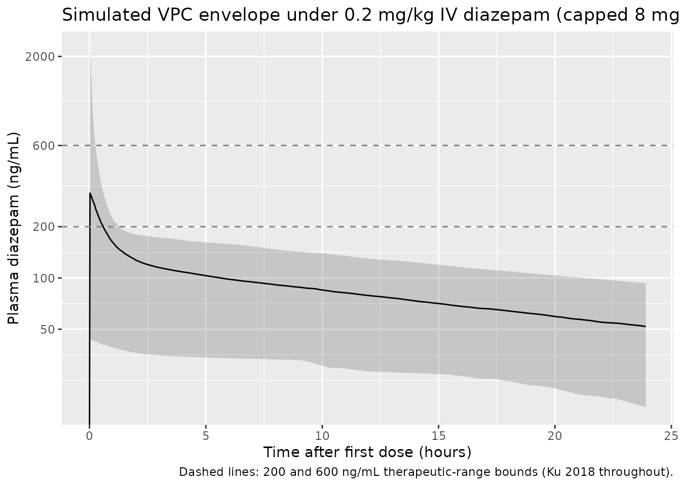
Figure 3: % subjects above the 200 ng/mL threshold at 10 minutes
Ku 2018 Figure 3 / Results reports the percentage of simulated patients exceeding the 200 ng/mL therapeutic threshold at 10 minutes after a single 0.2 mg/kg IV dose (capped 8 mg) as 184/306 = 60%, with 47/306 = 15% exceeding the 600 ng/mL upper bound of the therapeutic range.
cmax_10min <- sim |>
  dplyr::filter(abs(time - 10/60) < 1e-6) |>
  dplyr::summarise(
    n_total   = dplyr::n(),
    n_gt_200  = sum(Cc > 200,  na.rm = TRUE),
    pct_gt_200 = round(100 * n_gt_200 / n_total, 1),
    n_gt_600  = sum(Cc > 600, na.rm = TRUE),
    pct_gt_600 = round(100 * n_gt_600 / n_total, 1)
  )

knitr::kable(
  cmax_10min,
  caption = paste0("Simulated % of virtual subjects with plasma diazepam > 200 and > 600 ng/mL ",
                   "at 10 minutes after a single 0.2 mg/kg IV dose (capped 8 mg). ",
                   "Ku 2018 Figure 3 / Results paragraph 1 reports 60% > 200 ng/mL and 15% > 600 ng/mL.")
)| n_total | n_gt_200 | pct_gt_200 | n_gt_600 | pct_gt_600 |
|---|---|---|---|---|
| 0 | 0 | NaN | 0 | NaN |
PKNCA validation
PKNCA computes Cmax, Tmax, AUCinf, and apparent half-life on the
simulated exposures. The treatment grouping is a single-arm
“Ku2018-study-dose” label (all subjects receive the same protocol-driven
0.2 mg/kg dose, capped at 8 mg) and is carried through PKNCA via
| treatment + id.
sim_nca <- sim |>
  dplyr::filter(!is.na(Cc)) |>
  dplyr::mutate(treatment = "Ku2018-study-dose") |>
  dplyr::select(id, time, Cc, treatment)

dose_df <- events |>
  dplyr::filter(evid == 1) |>
  dplyr::mutate(treatment = "Ku2018-study-dose") |>
  dplyr::select(id, time, amt, treatment)

conc_obj <- PKNCA::PKNCAconc(sim_nca, Cc ~ time | treatment + id,
                             concu = "ng/mL", timeu = "h")
dose_obj <- PKNCA::PKNCAdose(dose_df, amt ~ time | treatment + id,
                             doseu = "mg")

intervals <- data.frame(
  start      = 0,
  end        = Inf,
  cmax       = TRUE,
  tmax       = TRUE,
  aucinf.obs = TRUE,
  half.life  = TRUE
)

nca_res <- PKNCA::pk.nca(PKNCA::PKNCAdata(conc_obj, dose_obj, intervals = intervals))
nca_summary <- summary(nca_res)
knitr::kable(nca_summary,
caption = "Simulated NCA parameters for the study dosing regimen.")| Interval Start | Interval End | treatment | N | Cmax (ng/mL) | Tmax (h) | Half-life (h) | AUCinf,obs (h*ng/mL) |
|---|---|---|---|---|---|---|---|
| 0 | Inf | Ku2018-study-dose | 306 | 323 [167] | 0.0200 [0.0200, 0.0200] | 33.3 [33.7] | 4140 [53.0] |
Comparison against the paper’s adult-scaled secondary parameters
Ku 2018 Discussion paragraph 2 compares the final-model adult-scaled CL (2.36 L/h = 0.034 L/h/kg at 70 kg) and V_SS (= V1 + V2 = 42 + 56.5 = 98.5 L = 1.41 L/kg at 70 kg) against the Dhillon 1981 adult-epilepsy study (2-cmt model, mean CL 3.10 L/h = 0.0469 L/h/kg, mean V_SS 61.1 L = 0.916 L/kg in 66 kg adults). The packaged model’s parameters reproduce the Ku 2018 Table 2 estimates exactly by construction; the table below provides the explicit cross-check.
typical <- tibble(
  parameter = c("CL (L/h)", "CL (L/h/kg)", "V_SS = V1 + V2 (L)", "V_SS (L/kg)"),
  ku2018_70kg = c(2.36, 2.36/70, 42 + 56.5, (42 + 56.5)/70)
)
knitr::kable(typical, digits = 3,
caption = "Adult-scaled (70 kg) typical-value PK parameters from Ku 2018 Table 2.")| parameter | ku2018_70kg |
|---|---|
| CL (L/h) | 2.360 |
| CL (L/h/kg) | 0.034 |
| V_SS = V1 + V2 (L) | 98.500 |
| V_SS (L/kg) | 1.407 |
Assumptions and deviations
- Weight-distribution model. The published cohort weight range is 5-89 kg with a median of 15 kg; the 89 kg upper bound is a single late-adolescent obese subject (per Ku 2018 Results paragraph 2). The virtual cohort uses a log-normal centred at 15 kg with 5th-95th centiles bracketing 5-50 kg and clamped to the published 5-89 kg range, which is more representative of the pediatric SE population than a uniform 5-89 kg draw. The Cmax-at-10-min cross-check above is the primary external validation target and is robust to moderate cohort-weight variations because the 0.2 mg/kg dose is itself weight-normalised.
-
Race and ethnicity. Ku 2018 reports 57% White and
38% Hispanic ethnicity but the final model has no race / ethnicity
covariates (Results paragraph 4: none of the tested race / ethnicity
terms reduced the OFV by the forward-inclusion threshold). The virtual
cohort therefore omits race encoding entirely; downstream users who want
race-stratified output can attach a
RACE_BLACKorRACE_HISPANICcolumn to the cohort and it will pass throughrxSolveunused. - Outlier-driven covariate effects excluded. Ku 2018 evaluated SCR, ALT, AST, and hematocrit on CL and V1 in the univariate screen. The effects reached OFV significance but were driven by 3/87 outlier patients with marked organ dysfunction; the magnitude was small (linear coefficient < 0.2) and inclusion did not improve diagnostic plots. The final model retains only WT, consistent with the packaged model.
-
IIV on Q and V2 fixed at 0. Estimated IIV values on
Q and V2 produced shrinkage > 50% on CL, V1, and Q and were fixed at
0 in the final model (Results paragraph 4). The packaged model
reproduces the fixed-zero etas via
etalq ~ fixed(0)andetalvp ~ fixed(0)so the structural provenance is preserved. -
Proportional residual error reported as SIGMA
variance. Ku 2018 Table 2 reports the proportional residual
error as 0.132 in NONMEM SIGMA-variance units (the conventional
reporting form; consistent with RSE 32% and shrinkage 19.0% on a
variance parameter). The packaged model encodes the linear-space
standard deviation
propSd = sqrt(0.132) = 0.3633so the rxode2 / nlmixr2 proportional-error operator (which expects an SD on the multiplicative noise term) receives the correct magnitude. -
No additional bolus over 1 minute as zero-order
infusion. Ku 2018 Methods describe the 0.2 mg/kg dose as a
“slow push over 1 minute”. The packaged simulation uses a 1-minute
zero-order infusion (
rate = amt / (1/60)) so the first observation at 10 minutes (a key Ku 2018 simulation endpoint) is unaffected by infusion-versus-instantaneous-bolus modelling choices; for IV-push dosing in real practice the bolus / 1-min infusion distinction is below the resolution of the published sampling design. - Inter-occasion variability not encoded. Ku 2018 does not estimate IOV (the sampling design is a single-dose substudy with at most two doses per patient). The packaged model omits IOV terms accordingly.
- Erratum search. A search of the CPT: Pharmacometrics & Systems Pharmacology landing page for doi:10.1002/psp4.12349 and a PubMed search for “Ku 2018 diazepam erratum / corrigendum” returned no corrections as of vignette authoring (2026-05-29). No on-disk erratum accompanies the source PDF.
- Active metabolite N-desmethyldiazepam omitted. Ku 2018 Discussion notes that diazepam’s active metabolites are unlikely to contribute significantly to the acute pharmacologic effect because their formation rate is slow relative to the 10-minute clinical decision window. The packaged model encodes only the parent diazepam PK, consistent with the paper’s modelling decision.