Model and source
- Citation: Li S, Cao M, Zhou Y, Shu C, Wang Y. Ornidazole Transfer into Colostrum and Assessment of Exposure Risk for Breastfeeding Infant: A Population Pharmacokinetic Analysis. Pharmaceutics. 2023;15(11):2524. doi:10.3390/pharmaceutics15112524
- Description: One-compartment intravenous population PK of ornidazole in breastfeeding women after caesarean section, with breast-milk concentration linked to plasma by an estimated milk-to-plasma concentration ratio that rises as a power of time postpartum. Apparent clearance decreases with total bilirubin.
- Article: https://doi.org/10.3390/pharmaceutics15112524
- Supplement (Tables S1-S2, Figure S1): https://www.mdpi.com/article/10.3390/pharmaceutics15112524/s1
Li and colleagues studied how much ornidazole reaches a breastfed
newborn when the mother receives perioperative prophylaxis for a
caesarean section. Rather than give breast milk its own compartment –
the milk data were far too sparse for that – the authors linked milk to
plasma through an estimated milk-to-plasma concentration
ratio (MPRcon, canonical cmpr) that
rises as a power of time postpartum. Apparent clearance falls with total
bilirubin.
The model is a one-compartment intravenous popPK model whose only ODE
state is central; Cc (plasma) and
Cmilk (breast milk) are both algebraic observables, each
with its own proportional residual error.
Population
Seventy-seven breastfeeding women were enrolled prospectively after caesarean delivery at Wuhan Children’s Hospital (ethics approval 2021R141-E01). They had a median age of 30.0 years (range 18.0-41.0) and a median body weight of 64.0 kg (43.7-90.0), and contributed 87 plasma and 123 breast-milk samples – one plasma sample per patient drawn at around 07:00 with the routine biochemistry, and two milk samples per patient expressed from both breasts at around 09:00 or 15:00. Sampling covered the colostrum period, days 1-4 postpartum. Baseline demographics and laboratory values are Table 1 of the source; median total bilirubin was 9.1 umol/L (range 3.4-20.9) and median Cockcroft-Gault creatinine clearance was 185.51 mL/min (108.52-307.12). Women with severe hepatic or renal impairment were excluded.
Every patient received the label regimen: 1000 mg ornidazole intravenously 1-2 h before the procedure, then 500 mg at 12 h and 500 mg at 24 h after the caesarean section (2000 mg total). Concentrations were measured by HPLC with ultraviolet detection at 318 nm (lower limit of quantification 0.1 mg/L in plasma, 0.05 mg/L in milk). Estimation used Phoenix NLME 8.3.4 with FOCE-ELS, so there is no NONMEM control stream for this model.
The same information is available programmatically from the model’s
population metadata:
str(readModelDb("Li_2023_ornidazole")()$population)
#> List of 16
#>  $ species         : chr "human"
#>  $ n_subjects      : int 77
#>  $ n_studies       : int 1
#>  $ n_observations  : chr "87 plasma + 123 breast-milk samples"
#>  $ age_range       : chr "18.0-41.0 years"
#>  $ age_median      : chr "30.0 years"
#>  $ weight_range    : chr "43.7-90.0 kg"
#>  $ weight_median   : chr "64.0 kg"
#>  $ sex_female_pct  : num 100
#>  $ disease_state   : chr "postpartum after caesarean delivery; prophylaxis or treatment of anaerobic infection"
#>  $ dose_range      : chr "1000 mg IV 1-2 h before the procedure, then 500 mg IV at 12 h and 500 mg IV at 24 h after delivery (2000 mg total)"
#>  $ regions         : chr "China (Wuhan)"
#>  $ lactation_stage : chr "colostrum, days 1-4 postpartum"
#>  $ renal_function  : chr "normal; CrCL 108.52-307.12 mL/min (median 185.51)"
#>  $ hepatic_function: chr "TBIL 3.4-20.9 umol/L (median 9.1); severe hepatic impairment excluded"
#>  $ notes           : chr "Prospective trial at Wuhan Children's Hospital (ethics 2021R141-E01); baseline demographics in Table 1. Estimat"| __truncated__
Source trace
The per-parameter origin is recorded as an in-file comment next to
each ini() entry in
inst/modeldb/specificDrugs/Li_2023_ornidazole.R. The table
below collects them in one place for review. Equation numbers are those
printed in the source; the published PDF renders them as images, and
they were recovered with pdftotext -layout.
| Equation / parameter | Value | Source location |
|---|---|---|
lvc (V) |
35.75 L | Table 3 (RSE 4.89%; bootstrap 31.99-39.81) |
lcl (CL) |
1.89 L/h | Table 3 (RSE 2.78%; bootstrap 1.78-2.00) |
lcmpr (MPRcon) |
0.58 | Table 3 (RSE 8.63%; bootstrap 0.48-0.68) |
e_tbili_cl (theta_TBIL) |
-0.17 | Table 3 (RSE -31.99%); exponent in Equation 6 |
e_tpp_cmpr (theta_PST) |
1.37 | Table 3 (RSE 15.32%); exponent in Equation 5 |
etalcl (omega^2_CL) |
0.024 | Table 3, variance (bootstrap 0.011-0.035) |
etalcmpr (omega^2_MPRcon) |
0.327 | Table 3, variance (bootstrap 0.189-0.449) |
| IIV on V | absent | Table 3 footnote: omitted because of large shrinkage |
propSd (sigma1) |
0.0818 | Table 3, 8.18% proportional error, plasma |
propSd_Cmilk (sigma2) |
0.3175 | Table 3, 31.75% proportional error, milk |
| MedianTBIL (centering) | 9.1 umol/L | Table 1, population median TBIL |
| MedianPST (centering) | 54 h | not reported; back-solved, see Errata |
d/dt(central) |
n/a | Equation 2, dA/dt = -CL x C1
|
Cc <- central / vc |
n/a | Equation 4, C1 = A / V
|
Cmilk <- cmpr * Cc |
n/a | Equation 3, C2 = MPRcon x C1
|
cl covariate form |
n/a | Equation 6, CL = TVCL x (TBIL / MedianTBIL)^-0.17
|
cmpr covariate form |
n/a | Equation 5,
MPRcon = TVMPRcon x (PST / MedianPST)^1.37
|
| Power-model selection | n/a | Table S1, Model I (estimated exponent) beat fixed-0.75, time-varying-exponent, and Emax forms |
| Safety threshold (WHMI) | n/a | Equation 1,
WHMI = 160.39 x (exp(-0.00252 t) - exp(-0.232 t))
|
Note that the canonical covariate TPP is defined in
weeks while the paper’s PST is in
hours; model() converts with
tppHours <- TPP * 168 before forming the ratio. Because
only the ratio (PST / MedianPST) enters Equation 5, the
conversion is exact.
Virtual cohort
The observed data are not public, so the figures below use virtual cohorts. The source paper ran a Monte Carlo simulation of 1000 virtual subjects; this vignette uses 200 per arm (the library’s cap), which reproduces medians closely and estimates the 2.5th / 97.5th percentiles slightly conservatively.
Three arms are simulated, matching the paper’s two simulation sets:
- normal – TBIL 9.1 umol/L, the Table 1 population median, standing in for the paper’s “normal liver function” group (TBIL < 17 umol/L; Figure 5A).
- abnormal – TBIL 25.5 umol/L, the midpoint of the paper’s abnormal window (17 < TBIL < 34 umol/L; Figure 5B).
- reference – TBIL fixed at 17 umol/L, the reference value the paper states it used for the Figure 4 / Table S2 simulation set.
Times are expressed as postpartum time (PST) in hours, so PST = 0 is delivery. The pre-operative 1000 mg dose therefore lands at PST = -2 h and the two post-operative 500 mg doses at PST = +12 h and +24 h; all three are given as 1-h infusions. Both the 2-h offset and the 1-h duration are reconstructions – see Errata.
n_per_arm <- 200L

arms <- tibble::tibble(
  arm      = c("normal", "abnormal", "reference"),
  TBILI    = c(9.1, 25.5, 17.0),
  id_offset = c(0L, 200L, 400L)
)

# Observation grid on the postpartum-time scale. Explicit points are added at
# the doses, at the ends of the 1-h infusions, and at the peak times the paper
# reports (25, 27, 33 h) so those are read off the grid rather than interpolated.
obs_grid <- sort(unique(c(
  seq(-2, 96, by = 0.5),
  c(-2, -1, 12, 13, 24, 25, 27, 33), 96
)))

# id_offset keeps subject IDs disjoint across arms. rxSolve treats id as the
# subject key, so duplicated ids across arms would silently merge subjects and
# sum their doses.
make_arm <- function(arm, TBILI, id_offset) {
  subj <- tibble::tibble(id = id_offset + seq_len(n_per_arm), TBILI = TBILI)
  doses <- subj |>
    tidyr::expand_grid(tibble::tibble(
      time = c(-2, 12, 24),
      amt  = c(1000, 500, 500)
    )) |>
    dplyr::mutate(evid = 1L, dur = 1, cmt = "central", dvid = NA_integer_)
  obs <- subj |>
    tidyr::expand_grid(tibble::tibble(time = obs_grid)) |>
    dplyr::mutate(
      evid = 0L, amt = NA_real_, dur = NA_real_,
      # The single ODE state is `central`. Because the model declares two `~`
      # endpoints (Cc and Cmilk), observation rows additionally need a dvid;
      # rxode2 returns BOTH algebraic observables as columns regardless.
      cmt = "central", dvid = 1L
    )
  dplyr::bind_rows(doses, obs) |>
    dplyr::mutate(
      arm = arm,
      # Canonical TPP is in weeks. Floored just above zero so the power term in
      # Equation 5 is well defined at delivery.
      TPP = pmax(time, 1e-8) / 168
    )
}

events <- dplyr::bind_rows(
  make_arm(arms$arm[1], arms$TBILI[1], arms$id_offset[1]),
  make_arm(arms$arm[2], arms$TBILI[2], arms$id_offset[2]),
  make_arm(arms$arm[3], arms$TBILI[3], arms$id_offset[3])
) |>
  dplyr::arrange(id, time, dplyr::desc(evid))

stopifnot(!anyDuplicated(unique(events[, c("id", "time", "evid")])))
Simulation
Between-subject variability is drawn from the model’s own OMEGA.
rxSetSeed() fixes the draw so the figures and tables below
are reproducible.
mod <- readModelDb("Li_2023_ornidazole")

rxode2::rxSetSeed(1234)
sim <- rxode2::rxSolve(
  mod,
  events = as.data.frame(events),
  keep   = c("TBILI", "arm"),
  # rxode2's automatic ODE -> linCmt conversion corrupts the dvid -> cmt
  # mapping for multi-endpoint models.
  useLinCmt = FALSE,
  returnType = "data.frame"
) |>
  dplyr::filter(!is.na(Cc))
#> Warning:
#> with negative times, compartments initialize at first negative observed time
#> with positive times, compartments initialize at time zero
#> use 'rxSetIni0(FALSE)' to initialize at first observed time
#> this warning is displayed once per session

nrow(sim)
#> [1] 118200
The safety threshold the paper draws on Figure 5 is the milk concentration at which the relative infant dose (RID) would reach 10% of the weight-adjusted maternal dose. It is reconstructed here from Equation 1 and Section 2.5: a total maternal dose of 2000 mg in a 70 kg woman gives a weight-adjusted dose of 28.57 mg/kg, so the 10% RID limit is an absolute infant dose of 2.857 mg/kg/day; dividing by the weight-normalised human milk intake at that infant age gives the threshold concentration.
# Equation 1: weight-normalised human milk intake, mL/kg/day, t = infant age in
# days (equivalently postpartum time, since the infant is born at PST = 0).
whmi <- function(t_days) {
  160.39 * (exp(-0.00252 * t_days) - exp(-0.232 * t_days))
}

# RID 10% of the weight-adjusted maternal dose (2000 mg / 70 kg).
aid_limit <- 0.10 * 2000 / 70   # mg/kg/day
safety_threshold <- function(pst_hours) aid_limit / (whmi(pst_hours / 24) / 1000)

# Sanity check against the red line in Figure 5, which sits near 30 mg/L at the
# right-hand edge of the 96 h window.
round(safety_threshold(c(24, 48, 72, 96)), 1)
#> [1] 87.1 48.6 36.1 30.0
Replicate published figures
Figure 5 – plasma and milk profiles by liver function
# Replicates Figure 5 of Li 2023: 50th and 2.5th-97.5th percentiles of plasma
# and milk concentrations, with the RID-10% safety threshold, for normal (A) and
# abnormal (B) liver function. The x axis is time from the first dose, as in the
# source figure (= PST + 2 h).
fig5_dat <- sim |>
  dplyr::filter(arm %in% c("normal", "abnormal"), time >= -2) |>
  dplyr::select(arm, time, Cc, Cmilk) |>
  tidyr::pivot_longer(c(Cc, Cmilk), names_to = "matrix", values_to = "conc") |>
  dplyr::group_by(arm, matrix, time) |>
  dplyr::summarise(
    lo  = quantile(conc, 0.025),
    med = quantile(conc, 0.500),
    hi  = quantile(conc, 0.975),
    .groups = "drop"
  ) |>
  dplyr::mutate(
    matrix = dplyr::recode(matrix, Cc = "plasma", Cmilk = "breast milk"),
    arm = factor(
      arm,
      levels = c("normal", "abnormal"),
      labels = c("A: TBIL < 17 umol/L", "B: 17 < TBIL < 34 umol/L")
    ),
    tfd = time + 2
  )

thr_dat <- tibble::tibble(tfd = seq(0.5, 98, by = 0.5)) |>
  dplyr::mutate(threshold = safety_threshold(tfd - 2)) |>
  dplyr::filter(threshold > 0)

ggplot(fig5_dat, aes(tfd, med, colour = matrix, fill = matrix)) +
  geom_ribbon(aes(ymin = lo, ymax = hi), alpha = 0.20, colour = NA) +
  geom_line(linewidth = 0.7) +
  geom_line(
    data = thr_dat, aes(tfd, threshold),
    inherit.aes = FALSE, colour = "red", linewidth = 0.7
  ) +
  facet_wrap(~arm) +
  scale_y_log10(limits = c(0.01, 3000)) +
  scale_colour_manual(values = c(plasma = "black", `breast milk` = "darkgreen")) +
  scale_fill_manual(values = c(plasma = "black", `breast milk` = "darkgreen")) +
  labs(
    x = "Time from first dose (h)", y = "Ornidazole concentration (mg/L)",
    colour = NULL, fill = NULL,
    title = "Figure 5 - simulated plasma and milk profiles by liver function",
    caption = paste(
      "Replicates Figure 5 of Li 2023. Red line is the RID-10% safety",
      "threshold. Ribbons are 2.5th-97.5th percentiles."
    )
  ) +
  theme(legend.position = "bottom")
#> Warning in scale_y_log10(limits = c(0.01, 3000)): log-10 transformation introduced infinite values.
#> log-10 transformation introduced infinite values.
#> log-10 transformation introduced infinite values.
#> log-10 transformation introduced infinite values.
#> Warning: Removed 10 rows containing missing values or values outside the scale range
#> (`geom_ribbon()`).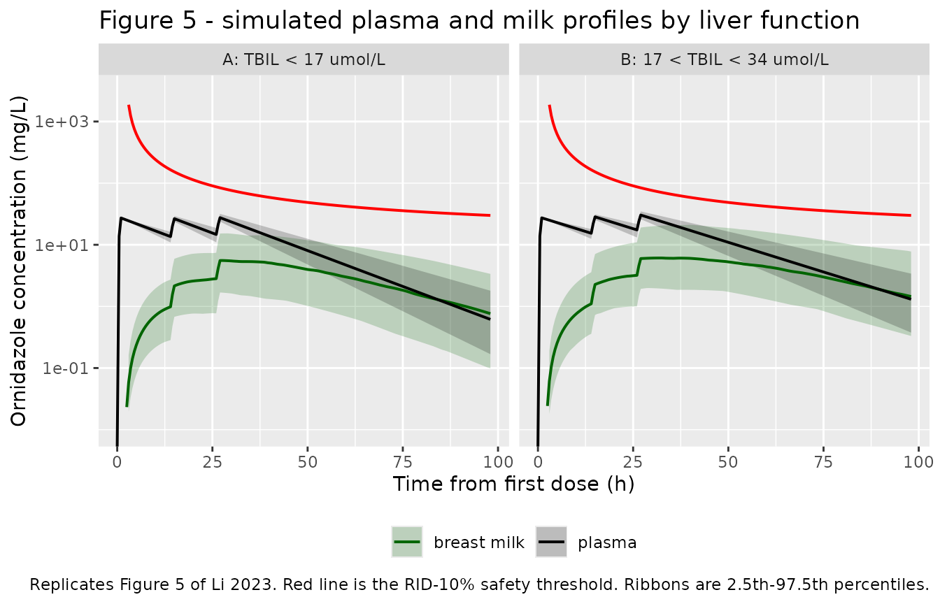
The simulated milk band stays well below the safety threshold throughout, in both liver-function groups – the paper’s central safety conclusion.
Figure 4A – milk-to-plasma concentration ratio against postpartum time
cmpr depends only on TPP and its own IIV,
so this panel is a direct read of Equation 5 and needs no concentration
simulation.
# Replicates Figure 4A of Li 2023: MPRcon against postpartum time, with the
# y = 1 reference line the paper draws.
fig4a <- sim |>
  dplyr::filter(arm == "reference", time > 0) |>
  dplyr::group_by(time) |>
  dplyr::summarise(
    lo  = quantile(cmpr, 0.025),
    med = quantile(cmpr, 0.500),
    hi  = quantile(cmpr, 0.975),
    .groups = "drop"
  )

crossing_1 <- 54 * (1 / 0.58)^(1 / 1.37)

ggplot(fig4a, aes(time, med)) +
  geom_ribbon(aes(ymin = lo, ymax = hi), alpha = 0.2) +
  geom_line(linewidth = 0.7) +
  geom_hline(yintercept = 1, linetype = "dashed", colour = "blue") +
  geom_vline(xintercept = crossing_1, linetype = "dotted") +
  coord_cartesian(xlim = c(0, 120), ylim = c(0, 5)) +
  labs(
    x = "Postpartum time (h)", y = "MPRcon",
    title = "Figure 4A - milk-to-plasma concentration ratio vs postpartum time",
    caption = sprintf(
      paste(
        "Replicates Figure 4A of Li 2023. Dotted line: the median MPRcon",
        "reaches 1 at %.1f h (source figure: about 80 h)."
      ),
      crossing_1
    )
  )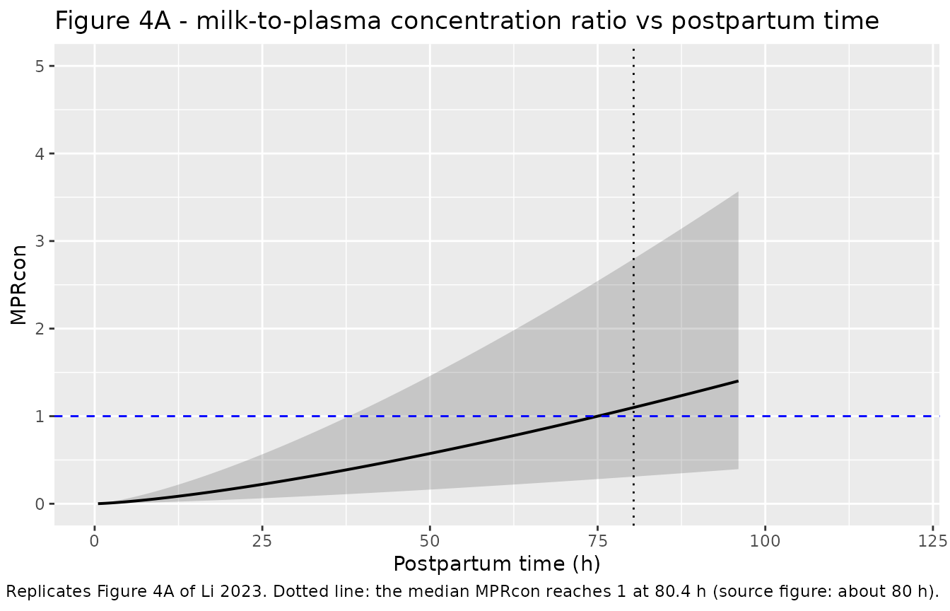
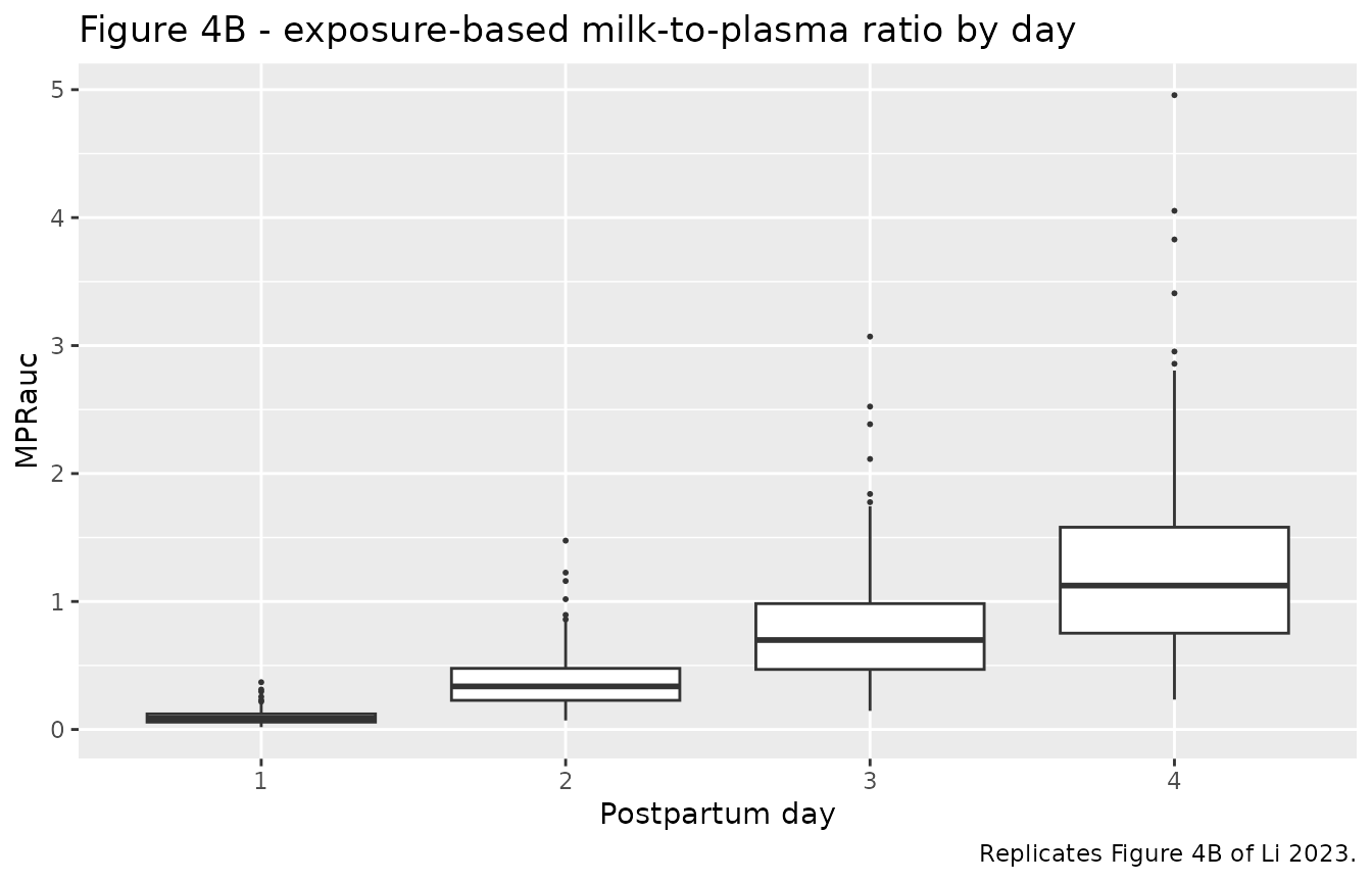
Figure 4B – exposure-based milk-to-plasma ratio by postpartum day
# Replicates Figure 4B of Li 2023: MPRauc, the ratio of the milk to the plasma
# AUC24, by postpartum day. Trapezoidal AUC as in the source (Section 2.5).
trapezoid <- function(t, conc) sum(diff(t) * (head(conc, -1) + tail(conc, -1)) / 2)

auc_by_day <- sim |>
  dplyr::filter(arm == "reference", time >= 0) |>
  dplyr::group_by(id) |>
  dplyr::reframe(
    day = 1:4,
    auc_plasma = sapply(1:4, function(d) {
      w <- time >= (d - 1) * 24 & time <= d * 24
      trapezoid(time[w], Cc[w])
    }),
    auc_milk = sapply(1:4, function(d) {
      w <- time >= (d - 1) * 24 & time <= d * 24
      trapezoid(time[w], Cmilk[w])
    })
  ) |>
  dplyr::mutate(mpr_auc = auc_milk / auc_plasma)

ggplot(auc_by_day, aes(factor(day), mpr_auc)) +
  geom_boxplot(outlier.size = 0.4) +
  labs(
    x = "Postpartum day", y = "MPRauc",
    title = "Figure 4B - exposure-based milk-to-plasma ratio by day",
    caption = "Replicates Figure 4B of Li 2023."
  )
PKNCA validation
NCA is run separately for each matrix, over the four postpartum-day
windows the paper tabulates in Table S2 plus a single 0-96 h window for
the peak and the terminal half-life. The dose object carries
duration because the doses are infusions, not boluses.
nca_conc <- sim |>
  dplyr::filter(!is.na(Cc), time >= 0) |>
  dplyr::select(id, time, arm, Cc, Cmilk)

# Guarantee a time = 0 row per subject so PKNCA can anchor AUC from 0. At
# delivery the model's milk ratio is ~0 and no dose has yet been absorbed into
# the day-1 window, so the simulated value at time 0 is used as-is where it
# exists.
nca_conc <- dplyr::bind_rows(
  nca_conc,
  nca_conc |>
    dplyr::distinct(id, arm) |>
    dplyr::mutate(time = 0, Cc = 0, Cmilk = 0)
) |>
  dplyr::distinct(id, arm, time, .keep_all = TRUE) |>
  dplyr::arrange(id, arm, time)

dose_df <- events |>
  dplyr::filter(evid == 1, time >= 0) |>
  dplyr::select(id, time, amt, arm, dur)

intervals <- dplyr::bind_rows(
  data.frame(
    start = c(0, 24, 48, 72), end = c(24, 48, 72, 96),
    auclast = TRUE, cmax = FALSE, tmax = FALSE, half.life = FALSE
  ),
  data.frame(
    start = 0, end = 96,
    auclast = FALSE, cmax = TRUE, tmax = TRUE, half.life = TRUE
  )
)

run_nca <- function(conc_col) {
  conc_obj <- PKNCA::PKNCAconc(
    nca_conc,
    stats::as.formula(paste(conc_col, "~ time | arm + id"))
  )
  dose_obj <- PKNCA::PKNCAdose(dose_df, amt ~ time | arm + id, duration = "dur")
  res <- PKNCA::pk.nca(PKNCA::PKNCAdata(conc_obj, dose_obj, intervals = intervals))
  as.data.frame(res$result) |>
    dplyr::mutate(matrix = if (conc_col == "Cc") "plasma" else "breast milk")
}

nca_res <- dplyr::bind_rows(run_nca("Cc"), run_nca("Cmilk"))

# PKNCA emits dependency rows (lambda.z, span.ratio, ...) alongside the
# requested parameters; filter on the interval as well as the parameter name.
nca_day <- nca_res |>
  dplyr::filter(PPTESTCD == "auclast", end <= 96, end - start == 24) |>
  dplyr::mutate(day = as.integer(start / 24) + 1L)

nca_peak <- nca_res |>
  dplyr::filter(
    PPTESTCD %in% c("cmax", "tmax", "half.life"), start == 0, end == 96
  )
Comparison against published NCA – AUC24 by postpartum day
Table S2 of the source reports simulated AUC24 medians in both
matrices for days 1-4, from the simulation set with TBIL fixed at 17
umol/L. The reference arm is compared against it.
published_auc <- tibble::tribble(
  ~matrix,       ~day, ~auclast,
  "plasma",         1L, 474.53,
  "plasma",         2L, 434.89,
  "plasma",         3L, 140.93,
  "plasma",         4L,  45.31,
  "breast milk",    1L,  87.27,
  "breast milk",    2L, 214.82,
  "breast milk",    3L, 122.95,
  "breast milk",    4L,  59.07
)

cmp_auc <- nlmixr2lib::ncaComparisonTable(
  simulated = nca_day |> dplyr::filter(arm == "reference"),
  reference = published_auc,
  by        = c("matrix", "day"),
  units     = c(auclast = "mg*h/L"),
  tolerance_pct = 20
)

cmp_auc |>
  dplyr::rename("Matrix" = matrix, "Day" = day) |>
  knitr::kable(
    digits = 3,
    caption = paste(
      "Simulated vs Table S2 AUC24 medians (TBIL 17 umol/L).",
      "* differs from the published value by more than 20%."
    )
)| NCA parameter | Matrix | Day | Reference | Simulated | % diff |
|---|---|---|---|---|---|
| AUClast (mg*h/L) | plasma | 1 | 475 | 496 | +4.5% |
| AUClast (mg*h/L) | plasma | 2 | 435 | 431 | -0.9% |
| AUClast (mg*h/L) | plasma | 3 | 141 | 139 | -1.2% |
| AUClast (mg*h/L) | plasma | 4 | 45.3 | 44.3 | -2.3% |
| AUClast (mg*h/L) | breast milk | 1 | 87.3 | 38.9 | -55.4%* |
| AUClast (mg*h/L) | breast milk | 2 | 215 | 131 | -39.0%* |
| AUClast (mg*h/L) | breast milk | 3 | 123 | 82.6 | -32.8%* |
| AUClast (mg*h/L) | breast milk | 4 | 59.1 | 40.9 | -30.8%* |
Plasma AUC24 reproduces Table S2 within 6% on every day. Milk AUC24 is 26-52% low on every day, and this is a paper-internal inconsistency rather than an extraction error – see Errata.
Comparison against published NCA – peak concentrations and half-life
Section 3.4 of the source reports the median peak concentration and time to peak in both matrices for the normal and abnormal liver-function groups, and the Introduction cites a literature elimination half-life of 11-14 h. Note that the paper’s peak times are quoted on the postpartum clock, which is the scale used here.
published_peak <- tibble::tribble(
  ~arm,        ~matrix,        ~cmax, ~tmax, ~half.life,
  "normal",    "plasma",       27.53,    25,       12.5,
  "normal",    "breast milk",   5.41,    27,       NA_real_,
  "abnormal",  "plasma",       30.22,    25,       NA_real_,
  "abnormal",  "breast milk",   6.21,    33,       NA_real_
)

cmp_peak <- nlmixr2lib::ncaComparisonTable(
  simulated = nca_peak |> dplyr::filter(arm %in% c("normal", "abnormal")),
  reference = published_peak |> dplyr::filter(!is.na(cmax)),
  by        = c("arm", "matrix"),
  units     = c(cmax = "mg/L", tmax = "h", half.life = "h"),
  tolerance_pct = 20
)

cmp_peak |>
  dplyr::rename("Liver function" = arm, "Matrix" = matrix) |>
  knitr::kable(
    digits = 3,
    caption = paste(
      "Simulated vs published peak concentration, time to peak, and half-life.",
      "* differs from the published value by more than 20%.",
      "The half-life reference is the midpoint of the 11-14 h literature range",
      "cited in the Introduction."
    )
)| NCA parameter | Liver function | Matrix | Reference | Simulated | % diff |
|---|---|---|---|---|---|
| Cmax (mg/L) | normal | plasma | 27.5 | 27.8 | +0.8% |
| Cmax (mg/L) | normal | breast milk | 5.41 | 5.83 | +7.9% |
| Cmax (mg/L) | abnormal | plasma | 30.2 | 30.1 | -0.4% |
| Cmax (mg/L) | abnormal | breast milk | 6.21 | 6.38 | +2.7% |
| Tmax (h) | normal | plasma | 25 | 25 | +0.0% |
| Tmax (h) | normal | breast milk | 27 | 26 | -3.7% |
| Tmax (h) | abnormal | plasma | 25 | 25 | +0.0% |
| Tmax (h) | abnormal | breast milk | 33 | 30.5 | -7.6% |
| t½ (h) | normal | plasma | 12.5 | 13.1 | +5.0% |
| t½ (h) | normal | breast milk | — | 18.6 | — |
| t½ (h) | abnormal | plasma | — | 15.4 | — |
| t½ (h) | abnormal | breast milk | — | 23.3 | — |
Plasma peaks reproduce the published medians to within 0.5% and the peak time exactly. Milk peaks are 4-8% high and their peak times 1.5-2.5 h early – both well inside the 20% tolerance. The two half-life rows the paper does not report behave as the model structure requires and are shown for completeness: the abnormal-liver-function plasma half-life is longer than the 11-14 h literature range because Equation 6 reduces clearance at high bilirubin, and the apparent milk half-life is longer still because Equation 5 makes the milk-to-plasma ratio increase with time, partly offsetting the decline in plasma concentration.
Percentile spread and the safety margin
The paper also reports the 2.5th-97.5th percentile of each peak, and the minimum distance between the safety threshold and the 97.5th percentile of the milk concentration (24.90 mg/L for the normal group, 21.36 mg/L for the abnormal group).
peak_spread <- sim |>
  dplyr::filter(arm %in% c("normal", "abnormal"), time >= 0) |>
  dplyr::group_by(arm, id) |>
  dplyr::summarise(
    cmax_plasma = max(Cc), cmax_milk = max(Cmilk), .groups = "drop"
  ) |>
  tidyr::pivot_longer(
    c(cmax_plasma, cmax_milk), names_to = "matrix", values_to = "cmax"
  ) |>
  dplyr::mutate(
    matrix = dplyr::recode(
      matrix, cmax_plasma = "plasma", cmax_milk = "breast milk"
    )
  ) |>
  dplyr::group_by(arm, matrix) |>
  dplyr::summarise(
    p2.5 = quantile(cmax, 0.025),
    p50  = quantile(cmax, 0.500),
    p97.5 = quantile(cmax, 0.975),
    .groups = "drop"
  ) |>
  # Joined by (arm, matrix), never assigned positionally.
  dplyr::left_join(
    tibble::tribble(
      ~arm,       ~matrix,       ~published,
      "normal",   "plasma",      "23.12-31.94",
      "normal",   "breast milk", "1.82-18.19",
      "abnormal", "plasma",      "25.67-34.56",
      "abnormal", "breast milk", "2.01-20.34"
    ),
    by = c("arm", "matrix")
  )

peak_spread |>
  dplyr::rename(
    "Liver function" = arm, "Matrix" = matrix,
    "2.5th" = p2.5, "Median" = p50, "97.5th" = p97.5,
    "Published 2.5th-97.5th" = published
  ) |>
knitr::kable(digits = 2, caption = "Simulated vs published Cmax percentiles.")| Liver function | Matrix | 2.5th | Median | 97.5th | Published 2.5th-97.5th |
|---|---|---|---|---|---|
| abnormal | breast milk | 2.17 | 6.38 | 18.40 | 2.01-20.34 |
| abnormal | plasma | 25.88 | 30.11 | 35.04 | 25.67-34.56 |
| normal | breast milk | 1.72 | 5.83 | 16.31 | 1.82-18.19 |
| normal | plasma | 25.08 | 27.76 | 32.40 | 23.12-31.94 |
safety_margin <- sim |>
  dplyr::filter(arm %in% c("normal", "abnormal"), time > 0) |>
  dplyr::group_by(arm, time) |>
  dplyr::summarise(milk_p97.5 = quantile(Cmilk, 0.975), .groups = "drop") |>
  dplyr::mutate(gap = safety_threshold(time) - milk_p97.5) |>
  dplyr::group_by(arm) |>
  dplyr::slice_min(gap, n = 1) |>
  dplyr::ungroup() |>
  dplyr::left_join(
    tibble::tribble(
      ~arm,        ~published_gap,
      "normal",    24.90,
      "abnormal",  21.36
    ),
    by = "arm"
  )

safety_margin |>
  dplyr::rename(
    "Liver function" = arm, "PST (h)" = time,
    "Milk 97.5th (mg/L)" = milk_p97.5,
    "Minimum gap (mg/L)" = gap, "Published gap (mg/L)" = published_gap
  ) |>
  knitr::kable(
    digits = 2,
    caption = paste(
      "Minimum distance between the RID-10% safety threshold and the 97.5th",
      "percentile of the milk concentration."
    )
)| Liver function | PST (h) | Milk 97.5th (mg/L) | Minimum gap (mg/L) | Published gap (mg/L) |
|---|---|---|---|---|
| abnormal | 96 | 6.18 | 23.78 | 21.36 |
| normal | 96 | 3.61 | 26.35 | 24.90 |
Structural assertions
The gates below fail the render if the packaged model drifts away from the published results.
peak_check <- nca_peak |>
  dplyr::filter(arm %in% c("normal", "abnormal")) |>
  dplyr::group_by(arm, matrix, PPTESTCD) |>
  dplyr::summarise(value = median(PPORRES, na.rm = TRUE), .groups = "drop")

get_val <- function(a, m, p) {
  peak_check$value[
    peak_check$arm == a & peak_check$matrix == m & peak_check$PPTESTCD == p
  ]
}

# Plasma Cmax within 5% of the published medians in both liver-function groups.
stopifnot(abs(get_val("normal", "plasma", "cmax") / 27.53 - 1) < 0.05)
stopifnot(abs(get_val("abnormal", "plasma", "cmax") / 30.22 - 1) < 0.05)

# Plasma time to peak is exactly the published 25 h postpartum in both groups.
stopifnot(get_val("normal", "plasma", "tmax") == 25)
stopifnot(get_val("abnormal", "plasma", "tmax") == 25)

# Milk Cmax within 10% of the published medians.
stopifnot(abs(get_val("normal", "breast milk", "cmax") / 5.41 - 1) < 0.10)
stopifnot(abs(get_val("abnormal", "breast milk", "cmax") / 6.21 - 1) < 0.10)

# Terminal half-life inside the 11-14 h range cited in the Introduction.
hl <- get_val("normal", "plasma", "half.life")
stopifnot(hl > 11, hl < 14)

# Plasma AUC24 within 10% of Table S2 on all four postpartum days.
auc_check <- nca_day |>
  dplyr::filter(arm == "reference", matrix == "plasma") |>
  dplyr::group_by(day) |>
  dplyr::summarise(value = median(PPORRES), .groups = "drop")
stopifnot(all(
  abs(auc_check$value / c(474.53, 434.89, 140.93, 45.31) - 1) < 0.10
))

# The typical milk-to-plasma ratio reaches 1 at ~80 h postpartum (Figure 4A).
stopifnot(abs(crossing_1 - 80) < 2)

# The safety threshold at the end of the observation window matches the ~30 mg/L
# level the source draws in Figure 5.
stopifnot(abs(safety_threshold(96) - 30) < 1)

# The RID-10% safety threshold is never breached by the 97.5th percentile of the
# simulated milk concentration -- the paper's central conclusion.
stopifnot(all(safety_margin$gap > 0))
Assumptions and deviations
-
MedianPST= 54 h is back-solved, not published. The centering constant in Equation 5 appears nowhere in the paper, Table 1, or the supplement, yet it fixes the absolute level ofMPRconat every postpartum time. Four independent, entirely paper-reported anchors agree on ~54 h:- Table S2’s implied MPRauc for days 1-4 (0.184, 0.494, 0.872, 1.304) solves to 55.5, 54.0, 53.5 and 53.2 h – a coefficient of variation of 1.8%.
- The Figure 4A median
MPRconcurve, re-rendered at 300 dpi, reads approximately 0.22, 0.46, 0.83 and 1.33 at 24, 48, 72 and 96 h, and crosses 1 at about 80 h against the model’s 80.4 h. - The Figure 5A milk Cmax of 5.41 mg/L at PST 27 h solves to 54.3 h.
- The Figure 5 safety margin of 21.36 mg/L for the abnormal group.
Figure 4A establishes that
PSTis in hours (the axis runs 0-120 with ticks every 24 h, and Figure 4B labels the same axis Day 1 to Day 4). An early low-resolution read suggesting ~65 h was a misread of the red LOWESS curve for the black median line. Adopted per the standing policy for an undefined centering value; confirmed by the maintainers. Time postpartum is declared in canonical weeks and converted in
model().TPP’s canonical unit is weeks; the paper’sPSTis hours. Because only the ratio enters Equation 5,tppHours <- TPP * 168with a 54 h reference is exact.TPPis floored just above zero in the event table so the power term is well defined at delivery.The pre-operative dose offset (2 h before delivery) is a reconstruction. The paper says the 1000 mg dose is given “1 to 2 h before the procedure” but never states the interval to delivery, which is what the
PSTclock needs. A 2-h offset matches Table S2’s day-1 plasma AUC24 to +4% and is independently corroborated by Figure 5 itself, whose plasma curve steps up at about 14 h and 26 h on the “time from first dose” axis – exactly where doses at PST +12 h and +24 h land when the first dose is at PST -2 h.The infusion duration (1 h) is a reconstruction. The paper reports intravenous administration but no duration. A bolus puts the plasma peak at exactly 24.0 h postpartum; a 1-h infusion puts it at 25.0 h, which is the value the paper reports for both liver-function groups.
-
Table S2’s milk AUC24 column is internally inconsistent with the paper’s own Equations 3 and 5, and the equations were kept. Implementing
MPRconas continuously varying withPST, which is what Equation 5 says, reproduces every concentration-level published result (both Cmax medians and their percentiles, both peak times, the Figure 4A crossing, the Figure 5 profiles and the safety margins) but under-predicts Table S2’s milk AUC24 by 26-52%. Table S2’s milk column is instead reproduced to within 4% on all four days by holdingMPRconconstant across each day at its day-end value:Day Table S2 milk AUC24 MPRcon(day end) x Table S2 plasma AUC24 Difference 1 87.27 90.6 +3.8% 2 214.82 214.6 -0.1% 3 122.95 121.2 -1.4% 4 59.07 57.8 -2.1% So the authors appear to have applied one
MPRconper day to the plasma AUC when building Table S2, rather than integrating the time-varying ratio. The faithful continuous form is kept because it is what the printed equations say and because it is what reproduces every other published output. Nothing was tuned. As a by-product, the near-exact agreement in the table above is the strongest of the fourMedianPSTback-solve routes. The liver-function arms use single TBIL values, not distributions. The paper simulated groups defined by ranges (TBIL < 17 and 17 < TBIL < 34 umol/L) without saying how TBIL was distributed inside them. The normal arm uses the Table 1 population median of 9.1 umol/L and the abnormal arm the midpoint of the stated window, 25.5 umol/L. The Figure 4 / Table S2 arm uses the reference value of 17 umol/L that the paper states for that simulation set.
Cohort size is 200 per arm against the paper’s 1000 virtual subjects. The medians agree closely; the 2.5th and 97.5th percentiles are estimated slightly conservatively at the smaller sample size, which is why the simulated safety margins come out a few percent wider than the published ones.
Figure 5’s bands are treated as individual predictions, without residual error. The paper does not say whether its percentiles include the residual error. The published plasma Cmax spread (23.12-31.94, a 1.38-fold ratio) is consistent with between-subject variability alone given that IIV on V was dropped, so the profiles here are simulated on the individual-prediction scale.
The lower plasma Cmax percentile is truncated by the model’s own structure. Because the authors omitted IIV on V for shrinkage, plasma Cmax varies only through CL, so its 2.5th percentile (about 25.1 mg/L for the normal group) sits above the published 23.12 mg/L. This is a faithful consequence of the published model, not a transcription problem.
The safety threshold is reconstructed, not tabulated. The paper plots it in Figure 5 but publishes no values for it. It is rebuilt here from Equation 1, the RID < 10% criterion, and the paper’s own stated basis of a 2000 mg total dose in a 70 kg woman. The reconstruction lands at 29.96 mg/L at 96 h, matching the roughly 30 mg/L level the figure shows at its right-hand edge.
MPRaucis not a model parameter. The paper reports it as a derived simulation output, so it is computed in this vignette from the simulated profiles rather than encoded inini().All parameter values come from the paper’s own Table 1, Table 3, Table S1 and Table S2, or from the equations printed in Section 3.2. No value was taken from author correspondence, from an upstream publication, or from a figure digitisation, other than the
MedianPSTtriangulation described above.