Phenytoin (Tanaka 2012)
Source:vignettes/articles/Tanaka_2012_phenytoin.Rmd
Tanaka_2012_phenytoin.RmdModel and source
- Citation: Tanaka J, Kasai H, Shimizu K, Shimasaki S, Kumagai Y. Population pharmacokinetics of phenytoin after intravenous administration of fosphenytoin sodium in pediatric patients, adult patients, and healthy volunteers. Eur J Clin Pharmacol. 2013;69(3):489-497. doi:10.1007/s00228-012-1373-8
- Description: Two-compartment population PK model for phenytoin after IV fosphenytoin sodium administration in Japanese healthy volunteers and adult / pediatric patients (Tanaka 2012). The fosphenytoin compartment converts first-order (K12) to the phenytoin central compartment; phenytoin is cleared from central and exchanges with a peripheral compartment via Q.
- Article: https://doi.org/10.1007/s00228-012-1373-8
Tanaka, Kasai, Shimizu, Shimasaki, and Kumagai (Bell Medical Solutions, Nobelpharma Co., and Kitasato University East Hospital) pooled data from two Japanese Phase I studies in healthy adult male volunteers and one Phase III study in adult and pediatric neurosurgical / epileptic patients to develop a two-compartment population PK model for phenytoin after intravenous administration of fosphenytoin sodium. The structural model (Figure 1) has a fosphenytoin compartment that converts first-order at rate K12 into the phenytoin central compartment; phenytoin is eliminated linearly from central and exchanges with a peripheral compartment via Q. Body weight enters as a power covariate on CL, V2 (central), and V3 (peripheral) with reference 60 kg. The model is used to recommend an adult fosphenytoin sodium dose of 22.5 mg/kg at 3 mg/kg/min for achieving the 10-20 ug/mL therapeutic range (Conclusions, page 495).
Population
The cohort included 71 subjects: 24 healthy adult male Japanese volunteers (two Phase I studies; ages 20-37, mean 24.9 years), 14 adult patients (Phase III; ages 17-86, mean 38.2 years; 7 male / 7 female; body weight 39.0-72.2 kg), and 33 pediatric patients (Phase III; ages 2-16, mean 7.8 years; 13 male / 20 female; body weight 7.8-60.3 kg). All subjects were Japanese. Adult and pediatric patients had status epilepticus, acute repetitive seizures, or required seizure prophylaxis after brain surgery / head trauma. A total of 923 plasma phenytoin concentrations were collected. Healthy volunteers received fixed doses of phenytoin sodium 250 mg or fosphenytoin sodium 375, 563, or 750 mg via 10-30 min IV infusions; patients received weight-banded fosphenytoin sodium 15, 18, or 22.5 mg/kg at 1 or 3 mg/kg/min (infusion duration capped at 150 mg/min total). Source: Tanaka 2012 Table 2 and Materials and methods - Study design (page 490).
The same information is available programmatically via the model’s
population metadata.
mod <- readModelDb("Tanaka_2012_phenytoin")
str(rxode2::rxode(mod)$population)
#> ℹ parameter labels from comments will be replaced by 'label()'
#> List of 11
#>  $ species       : chr "human"
#>  $ n_subjects    : int 71
#>  $ n_studies     : int 3
#>  $ age_range     : chr "2-86 years"
#>  $ weight_range  : chr "7.8-74.4 kg"
#>  $ sex_female_pct: num 38
#>  $ race_ethnicity: Named num 100
#>   ..- attr(*, "names")= chr "Asian"
#>  $ disease_state : chr "Pooled cohort of 24 healthy adult volunteers (Phase I crossover + Phase I dose-escalation), 14 adult patients ("| __truncated__
#>  $ dose_range    : chr "IV fosphenytoin sodium 375-750 mg (healthy volunteers, fixed doses) or 15-22.5 mg/kg (patients) infused at 8.3-"| __truncated__
#>  $ regions       : chr "Japan"
#>  $ notes         : chr "Tanaka 2012 Table 2 baseline demographics. Three pooled studies: two Phase I in healthy adult Japanese males (n"| __truncated__
Source trace
The per-parameter origin is recorded as an in-file comment next to
each ini() entry in
inst/modeldb/specificDrugs/Tanaka_2012_phenytoin.R. The
table below collects the same information in one place for review.
| Equation / parameter | Value at reference 60 kg | Source location |
|---|---|---|
lcl (CL, L/h) |
1.61 | Table 3 theta_1 |
lvc (V2, L) |
20.8 | Table 3 theta_3 |
lq (Q, L/h) |
53.0 | Table 3 theta_4 |
lvp (V3, L) |
26.0 | Table 3 theta_5 |
lka (K12, 1/h) |
5.02 | Table 3 theta_7 |
e_wt_cl |
0.569 | Table 3 theta_2; Equation 1 |
e_wt_vc |
1.0 (fixed) | Results page 494: “The influence factor of V2 was fixed to 1”; no theta entry in Table 3 |
e_wt_vp |
0.584 | Table 3 theta_6; Equation 1 |
etalcl (omega^2) |
0.194 | Table 3 omega_{CL,CL} |
etalvc (omega^2) |
0.161 | Table 3 omega_{V2,V2} |
etalq (omega^2) |
0.271 | Table 3 omega_{Q,Q} |
etalvp (omega^2) |
0.0430 | Table 3 omega_{V3,V3} |
etalka (omega^2) |
0.106 | Table 3 omega_{K12,K12} |
propSd (= sqrt(sigma_1^2)) |
sqrt(0.00148) = 0.0385 | Table 3 sigma_{1,1} = 0.00148 (variance) |
addSd (= sqrt(sigma_2^2)) |
sqrt(0.317) = 0.563 | Table 3 sigma_{2,2} = 0.317 (variance) |
Equation 1:
CL = theta_1 * (WT/60)^theta_2 * exp(eta_CL)
|
n/a | Eq. 1, page 494 |
Equation 1: V2 = theta_3 * (WT/60)^1 * exp(eta_V2)
|
n/a | Eq. 1, page 494 |
Equation 1:
V3 = theta_5 * (WT/60)^theta_6 * exp(eta_V3)
|
n/a | Eq. 1, page 494 |
Equation 1: Q = theta_4 * exp(eta_Q)
|
n/a | Eq. 1, page 494 |
Equation 1: K12 = theta_7 * exp(eta_K12)
|
n/a | Eq. 1, page 494 |
Residual error:
Y_ij = F_ij * exp(eps1_ij) + eps2_ij
|
n/a | Methods - Structural model, page 491 |
| Structural diagram (depot fosphenytoin -> central phenytoin via K12; central <-> peripheral via Q; CL from central) | n/a | Figure 1, page 491 |
Virtual cohort
The original observed data are not publicly available. The cohort below mirrors the Phase III adult patient population (body weight 53.5 +/- 9.9 kg) and reproduces the dose scenarios studied in the Tanaka 2012 Figure 5 dose simulation (adult fosphenytoin sodium 18, 22.5, and 30 mg/kg at 3 mg/kg/min constant infusion). Each treatment arm carries 200 simulated subjects to match the paper’s simulation design (“data sets of 200 subjects”; page 491).
set.seed(20120824)

# Adult cohort body weights resampled from N(53.5, 9.9^2), truncated to the
# Phase III range 39.0-72.2 kg per Tanaka 2012 Table 2 column 3.
sample_adult_wt <- function(n) {
  out <- numeric(0)
  while (length(out) < n) {
    candidate <- rnorm(n, mean = 53.5, sd = 9.9)
    keep <- candidate >= 39.0 & candidate <= 72.2
    out <- c(out, candidate[keep])
  }
  out[seq_len(n)]
}

make_cohort <- function(dose_mg_per_kg, infusion_rate_mg_per_kg_per_min,
                        n = 200L, t_end_h = 24, id_offset = 0L) {
  treatment_label <- sprintf("%.1f mg/kg @ %g mg/kg/min", dose_mg_per_kg,
                             infusion_rate_mg_per_kg_per_min)
  wt <- sample_adult_wt(n)
  total_dose_mg     <- dose_mg_per_kg * wt
  infusion_rate_mgh <- infusion_rate_mg_per_kg_per_min * wt * 60  # mg/h
  infusion_dur_h    <- total_dose_mg / infusion_rate_mgh
  ids <- id_offset + seq_len(n)
  # Dosing rows: rxode2 zero-order infusion uses rate > 0 with dur or amt.
  dose_rows <- tibble(
    id    = ids,
    time  = 0,
    evid  = 1L,
    cmt   = "depot",
    amt   = total_dose_mg,
    rate  = infusion_rate_mgh,
    WT    = wt,
    treatment = treatment_label
  )
  # Observation grid: dense around the infusion + early distribution phase,
  # then hourly out to t_end.
  obs_times <- sort(unique(c(seq(0, 1, by = 1/60),                  # 0-1 h, 1-min
                             seq(1, 4, by = 5/60),                  # 1-4 h, 5-min
                             seq(4, t_end_h, by = 0.25))))          # 4-24 h, 15-min
  obs_rows <- tidyr::expand_grid(
    id   = ids,
    time = obs_times
  ) |>
    mutate(evid = 0L, cmt = NA_character_, amt = 0, rate = 0) |>
    left_join(dose_rows |> select(id, WT, treatment), by = "id")
  bind_rows(dose_rows, obs_rows) |>
    arrange(id, time, desc(evid))
}

events <- bind_rows(
  make_cohort(18.0, 3, id_offset =   0L),
  make_cohort(22.5, 3, id_offset = 200L),
  make_cohort(30.0, 3, id_offset = 400L)
)

stopifnot(!anyDuplicated(unique(events[, c("id", "time", "evid")])))
Simulation
mod <- readModelDb("Tanaka_2012_phenytoin")
sim <- rxode2::rxSolve(
  mod,
  events = as.data.frame(events),
  keep   = c("WT", "treatment")
) |>
  as.data.frame()
#> ℹ parameter labels from comments will be replaced by 'label()'
head(sim)
#>   id       time       cl      vc        q       vp       ka       kel      k12
#> 1  1 0.00000000 1.472753 14.5429 55.47748 30.19675 3.566256 0.1012696 3.814747
#> 2  1 0.01666667 1.472753 14.5429 55.47748 30.19675 3.566256 0.1012696 3.814747
#> 3  1 0.03333333 1.472753 14.5429 55.47748 30.19675 3.566256 0.1012696 3.814747
#> 4  1 0.05000000 1.472753 14.5429 55.47748 30.19675 3.566256 0.1012696 3.814747
#> 5  1 0.06666667 1.472753 14.5429 55.47748 30.19675 3.566256 0.1012696 3.814747
#> 6  1 0.08333333 1.472753 14.5429 55.47748 30.19675 3.566256 0.1012696 3.814747
#>      k21        Cc  ipredSim        sim    depot  central peripheral1       WT
#> 1 1.8372 0.0000000 0.0000000 0.67309281   0.0000  0.00000  0.00000000 54.41109
#> 2 1.8372 0.3200765 0.3200765 0.05812154 158.4769  4.65484  0.09891009 54.41109
#> 3 1.8372 1.2291745 1.2291745 0.70647231 307.8087 17.87576  0.76151855 54.41109
#> 4 1.8372 2.6566247 2.6566247 2.80415998 448.5233 38.63502  2.47426509 54.41109
#> 5 1.8372 4.5391618 4.5391618 4.80747599 581.1178 66.01257  5.64801427 54.41109
#> 6 1.8372 6.8201940 6.8201940 7.01346439 706.0609 99.18539 10.62673762 54.41109
#>                  treatment
#> 1 18.0 mg/kg @ 3 mg/kg/min
#> 2 18.0 mg/kg @ 3 mg/kg/min
#> 3 18.0 mg/kg @ 3 mg/kg/min
#> 4 18.0 mg/kg @ 3 mg/kg/min
#> 5 18.0 mg/kg @ 3 mg/kg/min
#> 6 18.0 mg/kg @ 3 mg/kg/min
Replicate published figures
Figure 5 – simulated plasma phenytoin concentrations in adults
Tanaka 2012 Figure 5a-c shows simulated phenytoin concentration profiles over 24 h after single IV fosphenytoin doses of 18, 22.5, and 30 mg/kg at 3 mg/kg/min in adults, with the therapeutic range 10-20 ug/mL marked. The 95th and 5th percentile envelopes are drawn alongside individual subject profiles.
fig5_adults <- sim |>
  filter(time <= 24) |>
  group_by(treatment, time) |>
  summarise(
    Q05 = quantile(Cc, 0.05, na.rm = TRUE),
    Q50 = quantile(Cc, 0.50, na.rm = TRUE),
    Q95 = quantile(Cc, 0.95, na.rm = TRUE),
    .groups = "drop"
  )

ggplot(fig5_adults, aes(time, Q50)) +
  geom_ribbon(aes(ymin = Q05, ymax = Q95), alpha = 0.25) +
  geom_line(linewidth = 0.7) +
  geom_hline(yintercept = c(10, 20), linetype = "dotted", colour = "grey40") +
  facet_wrap(~ treatment, nrow = 1) +
  scale_y_continuous(limits = c(0, 70)) +
  labs(x = "Time (h)", y = "Total plasma phenytoin concentration (ug/mL)",
       title = "Figure 5 a-c -- Simulated adult plasma phenytoin",
       caption = "Replicates Figure 5 a-c of Tanaka 2012. Dotted lines = therapeutic range 10-20 ug/mL.")
#> Warning: Removed 1 row containing missing values or values outside the scale range
#> (`geom_ribbon()`).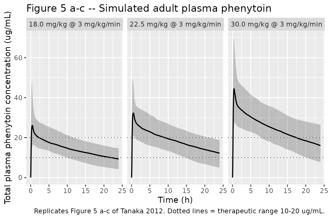
At 18 mg/kg the concentration drops below the 10 ug/mL lower bound within a few hours; at 22.5 mg/kg the typical-value profile stays within the therapeutic range across most of the 24-h window (consistent with the paper’s Conclusion that 22.5 mg/kg at 3 mg/kg/min is the optimal adult dose); at 30 mg/kg the Cmax exceeds the 20 ug/mL toxic threshold in essentially all simulated subjects (Tanaka 2012 Results, page 495).
Fosphenytoin to phenytoin conversion half-life
Tanaka 2012 reports an estimated fosphenytoin to phenytoin conversion half-life of approximately 8 minutes, derived from K12 (Discussion, page 495: “The estimated half-life of conversion from fosphenytoin to phenytoin calculated from K12, which was approximately 8 min, was consistent with the half-life proposed by Boucher et al.”). With K12 = 5.02 1/h:
PKNCA validation
Single-dose NCA over the 24-h post-infusion window per Recipe 1 in
references/pknca-recipes.md, stratified by treatment
arm.
sim_nca <- sim |>
  filter(!is.na(Cc)) |>
  select(id, time, Cc, treatment)

dose_df <- events |>
  filter(evid == 1) |>
  select(id, time, amt, treatment)

conc_obj <- PKNCA::PKNCAconc(
  as.data.frame(sim_nca), Cc ~ time | treatment + id,
  concu = "ug/mL", timeu = "h"
)
dose_obj <- PKNCA::PKNCAdose(
  as.data.frame(dose_df), amt ~ time | treatment + id,
  doseu = "mg"
)

intervals <- data.frame(
  start      = 0,
  end        = 24,
  cmax       = TRUE,
  tmax       = TRUE,
  auclast    = TRUE,
  half.life  = TRUE
)

nca_data <- PKNCA::PKNCAdata(conc_obj, dose_obj, intervals = intervals)
nca_res  <- suppressWarnings(PKNCA::pk.nca(nca_data))
nca_tbl  <- as.data.frame(nca_res$result)

nca_summary <- nca_tbl |>
  filter(PPTESTCD %in% c("cmax", "tmax", "auclast", "half.life")) |>
  group_by(treatment, PPTESTCD) |>
  summarise(
    median = median(PPORRES, na.rm = TRUE),
    q05    = quantile(PPORRES, 0.05, na.rm = TRUE),
    q95    = quantile(PPORRES, 0.95, na.rm = TRUE),
    .groups = "drop"
  )
knitr::kable(nca_summary, digits = 3,
caption = "Single-dose NCA over 0-24 h by adult dose arm (n = 200 each).")| treatment | PPTESTCD | median | q05 | q95 |
|---|---|---|---|---|
| 18.0 mg/kg @ 3 mg/kg/min | auclast | 355.146 | 231.560 | 492.407 |
| 18.0 mg/kg @ 3 mg/kg/min | cmax | 26.556 | 18.282 | 41.276 |
| 18.0 mg/kg @ 3 mg/kg/min | half.life | 21.090 | 8.863 | 46.873 |
| 18.0 mg/kg @ 3 mg/kg/min | tmax | 0.433 | 0.250 | 0.784 |
| 22.5 mg/kg @ 3 mg/kg/min | auclast | 434.650 | 308.048 | 599.174 |
| 22.5 mg/kg @ 3 mg/kg/min | cmax | 33.626 | 22.175 | 54.335 |
| 22.5 mg/kg @ 3 mg/kg/min | half.life | 20.788 | 8.645 | 51.982 |
| 22.5 mg/kg @ 3 mg/kg/min | tmax | 0.417 | 0.283 | 1.004 |
| 30.0 mg/kg @ 3 mg/kg/min | auclast | 576.492 | 403.112 | 826.593 |
| 30.0 mg/kg @ 3 mg/kg/min | cmax | 44.409 | 27.682 | 71.377 |
| 30.0 mg/kg @ 3 mg/kg/min | half.life | 20.272 | 8.721 | 40.847 |
| 30.0 mg/kg @ 3 mg/kg/min | tmax | 0.450 | 0.317 | 0.951 |
Comparison against published figures
Tanaka 2012 does not publish a NCA table; the validation target is therefore the visual envelope in Figure 5. The 95th-percentile Cmax in the simulated output should match the paper’s Figure 5 envelopes:
- 18 mg/kg – Cmax envelope below the 20 ug/mL toxic threshold; medians drop below 10 ug/mL within the first few hours.
- 22.5 mg/kg – 95th-percentile Cmax modestly exceeds 20 ug/mL; the typical profile remains close to the 10-20 ug/mL band over the 24-h window.
- 30 mg/kg – 95th-percentile Cmax well above 20 ug/mL; even the 5th percentile reaches the toxic threshold (Results, page 495: “Cmax values were more than 20 ug/mL in almost all simulations at a dose of 30 mg/kg”).
sim |>
  group_by(treatment, id) |>
  summarise(Cmax = max(Cc, na.rm = TRUE), .groups = "drop") |>
  group_by(treatment) |>
  summarise(
    median_Cmax = median(Cmax),
    q05_Cmax    = quantile(Cmax, 0.05),
    q95_Cmax    = quantile(Cmax, 0.95),
    pct_over_20 = 100 * mean(Cmax > 20),
    .groups = "drop"
  ) |>
  knitr::kable(digits = 2,
caption = "Per-subject Cmax envelope and percent of subjects with Cmax > 20 ug/mL toxic threshold.")| treatment | median_Cmax | q05_Cmax | q95_Cmax | pct_over_20 |
|---|---|---|---|---|
| 18.0 mg/kg @ 3 mg/kg/min | 26.56 | 18.28 | 41.28 | 88.0 |
| 22.5 mg/kg @ 3 mg/kg/min | 33.63 | 22.17 | 54.33 | 96.5 |
| 30.0 mg/kg @ 3 mg/kg/min | 44.41 | 27.68 | 71.38 | 99.5 |
Assumptions and deviations
-
Pediatric arm not reproduced in this vignette.
Tanaka 2012 Figure 5 panels d-f show pediatric simulations at the same
18 / 22.5 / 30 mg/kg doses, with covariates resampled from the Phase III
pediatric cohort. The packaged model handles pediatric patients
identically – the allometric power-law on WT is valid across the
7.8-74.4 kg observed range – but the vignette restricts to the adult arm
to keep figure replication focused. Users can substitute a
sample_pediatric_wt()helper drawing fromN(24.4, 13.0^2)truncated to 7.8-60.3 kg (Tanaka 2012 Table 2 column 4) to reproduce the pediatric panels. -
Residual error variance reported as
sigma^2, encoded assqrt(sigma^2)on SD scale. Tanaka 2012 Table 3 reports residual errors as variances (column headersigma^2). nlmixr2’sprop()andadd()error functions use SD; the model file converts viapropSd = sqrt(0.00148) = 0.0385andaddSd = sqrt(0.317) = 0.5630 ug/mL. The combined exponential + additive formY = F * exp(eps1) + eps2(page 491) linearizes toY ~ F * (1 + eps1) + eps2for small eps1, mapping to theprop(propSd) + add(addSd)combination used here. -
Inter-individual variability covariances zero.
Tanaka 2012 Table 3 reports only diagonal entries
(
omega_{CL,CL},omega_{V2,V2},omega_{Q,Q},omega_{V3,V3},omega_{K12,K12}); the off-diagonals are not estimated and are treated as zero in this implementation. -
Bioavailability of phenytoin from IV fosphenytoin assumed to
be 1. Tanaka 2012 Structural model (page 491) states “The
bioavailability of phenytoin derived from intravenous fosphenytoin
sodium injection is approximately 1.” No explicit
F1is fit; the model file therefore omits anlfdepotterm and the depot-to-central first-order conversion implicitly carries the 1:1 mass conversion that the paper’s parameters assume. -
Direct IV phenytoin administration (Phase I crossover arm)
requires dataset-level
cmttargeting central. The Phase I crossover study (page 490) dosed phenytoin sodium 250 mg IV directly without the fosphenytoin prodrug step. To simulate that scenario, setcmt = "central"on the corresponding dose record so the dose bypasses the depot (fosphenytoin) compartment. -
Dose units are mg of fosphenytoin sodium. The model
is parameterised to the paper’s reported doses (mg of fosphenytoin
sodium), not phenytoin equivalents. The K12 conversion step implicitly
absorbs the molecular weight ratio that Tanaka 2012 did not explicitly
fit; users who wish to dose in phenytoin equivalents (PE) should scale
the input amount by the appropriate conversion factor before passing to
rxSolve.