Ropinirole (Kaikousidis 2024)
Source:vignettes/articles/Kaikousidis_2024_ropinirole.Rmd
Kaikousidis_2024_ropinirole.RmdModel and source
- Citation: Kaikousidis C, Bies RR, Dokoumetzidis A. Simulating realistic patient profiles from pharmacokinetic models by a machine learning postprocessing correction of residual variability. CPT Pharmacometrics Syst Pharmacol. 2024;13(9):1476-1487. doi:10.1002/psp4.13182.
- Article: https://doi.org/10.1002/psp4.13182 (open access; the population parameter estimates are in Supplementary Tables S2 and S3 of Data S1)
Kaikousidis 2024 is a methods paper: it proposes a machine-learning (random forest) correction of the individual residual errors of a population PK model, so that simulated individual profiles look like real ones. The method was applied to two population PK models of ropinirole fitted in Monolix to the same dense single-dose dataset. Both are packaged here:
-
Kaikousidis_2024_ropinirole– the final model (Model 1): One-compartment population PK model for ropinirole after a single 2 mg oral dose of a prolonged-release tablet (Requip) in healthy adult volunteers (Kaikousidis 2024, final Model 1). Linear elimination and a double absorption: a fraction F1 of the dose passes through a Savic transit-compartment chain (mean transit time Mtt1, transit rate constant Ktr1, non-integer number of transits Mtt1 * Ktr1 - 1) into an absorption compartment emptied with first-order rate ka1, while the remaining 1 - F1 is absorbed simultaneously with first-order rate ka2 after a lag time Tlag2 = Mtt1 + diffTlag2 that always exceeds the mean transit time. Log-normal IIV on all structural parameters and logit-normal IIV on F1; proportional residual error. Each dose is given as two event records, one into depot and one into depot2, with the same amount. -
Kaikousidis_2024_ropinirole_misspecified– the earlier, simpler model (Model 2) that the authors kept as a heavily misspecified comparator: One-compartment population PK model for ropinirole after a single 2 mg oral dose of a prolonged-release tablet (Requip) in healthy adult volunteers (Kaikousidis 2024, Model 2). This is the earlier, simpler model the authors kept as a deliberately misspecified comparator: it does not capture the second concentration peak, and its proportional residual error (0.33) is larger than that of the final model (Kaikousidis_2024_ropinirole). Linear elimination and a double first-order absorption without lag times: a fraction F1 of the dose is absorbed with rate ka1 and the remaining 1 - F1 simultaneously with rate ka2. Log-normal IIV on ka1, ka2, V and CL and logit-normal IIV on F1; proportional residual error. Each dose is given as two event records, one into depot and one into depot2, with the same amount.
The machine-learning correction itself is a trained random-forest object (published by the authors on GitHub, PMXathens/MLRopinirole) applied to the model output after simulation; it is not part of either model and is not reproduced here.
Population
Thirty healthy volunteers received a single oral 2 mg dose of a prolonged-release ropinirole tablet (Requip, GlaxoSmithKline), with 18 plasma samples per subject at 0, 1, 2, 3, 4, 5, 6, 7, 8, 9, 10, 12, 14, 16, 18, 24, 36, 48 and 60 h (Supplementary Information, Dataset). Mean (SD) age was 32 (8) years (range 19-44), weight 74.5 (10.3) kg (range 54.7-94.8), height 172.3 (8.0) cm and BMI 25.1 (2.7) kg/m^2; 73.3% were male. The cohort was 56.6% Black, 20% Caucasian, 10% Asian and 13.4% other (Supplementary Table S1). Neither model has covariates.
The same information is available programmatically via
readModelDb("Kaikousidis_2024_ropinirole")()$population.
Source trace
All values are from the Monolix population parameter tables in the
supplement. Monolix reports each omega as the standard
deviation of the random effect on the transformed scale; the packaged
variances are omega^2.
Model 1 (final model, Supplementary Table S2)
| Parameter | Packaged value | Source |
|---|---|---|
lka (ka1) |
log(0.09886) 1/h |
Table S2 ka1_pop
|
lka2 (ka2) |
log(0.2501) 1/h |
Table S2 ka2_pop
|
logitfdepot (F1) |
logit(0.8071) |
Table S2 F1_pop
|
lmtt (Mtt1) |
log(0.5545) h |
Table S2 Mtt1_pop
|
lktr (Ktr1) |
log(1.8352) 1/h |
Table S2 Ktr1_pop
|
ldtlag2 (diffTlag2) |
log(11.985) h |
Table S2 diffTlag2_pop
|
lvc (V) |
log(311.7171) L |
Table S2 V_pop
|
lcl (Cl) |
log(72.2331) L/h |
Table S2 Cl_pop
|
etalka, etalka2,
etalogitfdepot, etalmtt, etalktr,
etaldtlag2, etalvc, etalcl
|
0.2076^2, 0.1657^2, 0.5086^2, 0.544^2, 1.8695^2, 0.1956^2, 0.2014^2, 0.3539^2 | Table S2 omega_*
|
propSd |
0.222 | Table S2 Prop. RUV
|
| Double absorption: transit arm (fraction F1, Mtt1, Ktr1, ka1) plus simultaneous first-order arm (1 - F1, ka2) | n/a | Results, “Modeling the residual error” |
tlag2 <- mtt + dtlag2 |
n/a | Results, “Tlag2 = Mtt1 + diffTlag2” |
| One compartment, linear elimination | n/a | Results, “Modeling the residual error” |
Model 2 (misspecified model, Supplementary Table S3)
| Parameter | Packaged value | Source |
|---|---|---|
lka (ka1) |
log(0.1214) 1/h |
Table S3 ka1_pop
|
lka2 (ka2) |
log(0.2614) 1/h |
Table S3 ka2_pop
|
logitfdepot (F1) |
logit(0.9987) |
Table S3 F1_pop
|
lvc (V) |
log(653.4056) L |
Table S3 V_pop
|
lcl (Cl) |
log(80.0181) L/h |
Table S3 Cl_pop
|
etalka, etalka2,
etalogitfdepot, etalvc,
etalcl
|
0.1737^2, 1.715^2, 0.6061^2, 0.1805^2, 0.3426^2 | Table S3 omega_*
|
propSd |
0.3293 | Table S3 Prop. RUV
|
| Double first-order absorption (F1 with ka1, 1 - F1 with ka2), no lag | n/a | Results, “Modeling the residual error” |
Transit absorption in Model 1
Monolix’s transit-compartment absorption (parameters Mtt, Ktr, ka)
has a non-integer number of transit compartments
nn = Mtt * Ktr - 1, and the flow into the absorption
compartment is the Savic gamma density with shape nn + 1
and rate Ktr. Because of the very large IIV on Ktr1 (omega
1.87), nn lies between -1 and 0 for about half the
subjects; the density is then unbounded at the dose time and an ODE
solver cannot integrate it. The packaged model uses the equivalent
integrated form instead: depot holds all transit-arm drug
not yet absorbed, the part still in the transit chain is
F1 * dose * (1 - P(nn + 1, Ktr * tad)) (with P
the regularized lower incomplete gamma function, rxode2’s
gammap()), and only the remainder is absorbed with rate
ka1.
The check below solves both forms for fixed parameter sets with
nn > 0, where the gamma-density form can be integrated,
and requires them to agree.
mod1 <- readModelDb("Kaikousidis_2024_ropinirole")
mod2 <- readModelDb("Kaikousidis_2024_ropinirole_misspecified")

# Gamma-density (Savic kernel) form of the Model 1 structure, as a plain
# rxode2 model with every parameter supplied directly.
kernel_form <- rxode2::rxode2({
  nn <- mtt * ktr - 1
  inp <- 0
  if (t > 0) {
    inp <- fdepot * dose * exp((nn + 1) * log(ktr) + nn * log(t) - ktr * t - lgamma(nn + 1))
  }
  d/dt(depot) <- inp - ka * depot
  d/dt(depot2) <- -ka2 * depot2
  d/dt(central) <- ka * depot + ka2 * depot2 - cl / vc * central
  f(depot) <- 0
  f(depot2) <- 1 - fdepot
  alag(depot2) <- tlag2
  Cc <- 1e6 * central / vc
})

# Parameter sets spanning short and long transit chains (nn = 0.5, 3 and 12).
check_par <- tibble(
  id = 1:3, ka = 0.09886, ka2 = 0.2501, fdepot = 0.8071, vc = 311.7171,
  cl = 72.2331, mtt = c(0.5545, 1.5, 3), ktr = c(1.5, 4, 13) / mtt,
  dtlag2 = 11.985
) |>
  mutate(tlag2 = mtt + dtlag2)

check_times <- c(0, seq(0.25, 72, by = 0.25))
check_ev <- bind_rows(
  tidyr::expand_grid(id = 1:3, cmt = c("depot", "depot2")) |>
    mutate(time = 0, amt = 2, evid = 1L),
  tidyr::expand_grid(id = 1:3, time = check_times) |>
    mutate(cmt = "central", amt = NA_real_, evid = 0L)
) |>
  arrange(id, time, desc(evid))

kernel_sim <- rxode2::rxSolve(
  kernel_form, left_join(check_ev, check_par, by = "id") |> mutate(dose = 2),
  method = "dop853", atol = 1e-12, rtol = 1e-12, maxsteps = 1e6L,
  returnType = "data.frame"
)

# The packaged model with the same individual parameters: zero the etas and
# replace the typical values with each subject's parameters.
mod1_typical <- rxode2::zeroRe(mod1)
#> ℹ parameter labels from comments will be replaced by 'label()'
packaged_sim <- bind_rows(lapply(seq_len(nrow(check_par)), function(i) {
  p <- check_par[i, ]
  theta <- c(
    lka = log(p$ka), lka2 = log(p$ka2), logitfdepot = rxode2::logit(p$fdepot),
    lmtt = log(p$mtt), lktr = log(p$ktr), ldtlag2 = log(p$dtlag2),
    lvc = log(p$vc), lcl = log(p$cl)
  )
  rxode2::rxSolve(mod1_typical, check_ev |> filter(id == p$id), params = theta,
                  atol = 1e-10, rtol = 1e-10, returnType = "data.frame") |>
    mutate(id = p$id)
}))
#> ℹ omega/sigma items treated as zero: 'etalka', 'etalka2', 'etalogitfdepot', 'etalmtt', 'etalktr', 'etaldtlag2', 'etalvc', 'etalcl'
#> ℹ omega/sigma items treated as zero: 'etalka', 'etalka2', 'etalogitfdepot', 'etalmtt', 'etalktr', 'etaldtlag2', 'etalvc', 'etalcl'
#> ℹ omega/sigma items treated as zero: 'etalka', 'etalka2', 'etalogitfdepot', 'etalmtt', 'etalktr', 'etaldtlag2', 'etalvc', 'etalcl'

transit_cmp <- inner_join(
  kernel_sim |> select(id, time, Cc_kernel = Cc),
  packaged_sim |> select(id, time, Cc_packaged = Cc),
  by = c("id", "time")
)
stopifnot(nrow(transit_cmp) == 3 * length(check_times))
max_rel_diff <- max(abs(transit_cmp$Cc_packaged - transit_cmp$Cc_kernel) /
                      max(transit_cmp$Cc_kernel))
max_rel_diff
#> [1] 3.328343e-09
# Measured about 3e-9; both solves are deterministic.
stopifnot(max_rel_diff < 1e-4)
Virtual cohort and simulation
The observed data are not public. The simulations use 200 virtual
subjects per model, each receiving a single 2 mg dose at time 0. Each
dose is entered as two event records with the full amount, one into
depot and one into depot2; the models split it
between the two absorption arms with f(). Neither model has
covariates, so the cohort needs no demographics.
n_sub <- 200
obs_times <- sort(unique(c(seq(0, 60, by = 0.5), 0:10, 12, 14, 16, 18, 24, 36, 48, 60)))

make_events <- function(n, treatment, id_offset = 0L) {
  ids <- id_offset + seq_len(n)
  bind_rows(
    tidyr::expand_grid(id = ids, cmt = c("depot", "depot2")) |>
      mutate(time = 0, amt = 2, evid = 1L),
    tidyr::expand_grid(id = ids, time = obs_times) |>
      mutate(cmt = "central", amt = NA_real_, evid = 0L)
  ) |>
    mutate(treatment = treatment) |>
    arrange(id, time, desc(evid))
}

ev1 <- make_events(n_sub, "Model 1 (final)")
ev2 <- make_events(n_sub, "Model 2 (misspecified)", id_offset = n_sub)
stopifnot(!anyDuplicated(unique(bind_rows(ev1, ev2)[, c("id", "time", "evid", "cmt")])))
rxode2::rxSetSeed(20241182)
sim1 <- rxode2::rxSolve(mod1, ev1, keep = "treatment", returnType = "data.frame")
#> ℹ parameter labels from comments will be replaced by 'label()'
rxode2::rxSetSeed(20241183)
sim2 <- rxode2::rxSolve(mod2, ev2, keep = "treatment", returnType = "data.frame")
#> ℹ parameter labels from comments will be replaced by 'label()'
sim <- bind_rows(sim1, sim2)

# Every subject solves, and the transit-arm depot never goes negative.
stopifnot(!anyNA(sim$ipredSim))
stopifnot(min(sim1$depot) >= -1e-6 * 2)
Replicate published figures
Figures 3(a) and 4(a) of the paper are visual predictive checks of the uncorrected models (10th, 50th and 90th percentiles). The plot below shows the same percentiles of the simulated observations (individual predictions with proportional residual error).
vpc <- sim |>
  group_by(treatment, time) |>
  summarise(
    p10 = quantile(sim, 0.10),
    p50 = quantile(sim, 0.50),
    p90 = quantile(sim, 0.90),
    .groups = "drop"
  )

ggplot(vpc, aes(time)) +
  geom_ribbon(aes(ymin = p10, ymax = p90), fill = "steelblue", alpha = 0.2) +
  geom_line(aes(y = p50), colour = "steelblue4") +
  geom_line(aes(y = p10), colour = "firebrick", linetype = "dashed") +
  geom_line(aes(y = p90), colour = "firebrick", linetype = "dashed") +
  facet_wrap(~treatment) +
  labs(
    x = "Time (h)", y = "Ropinirole concentration (ng/L)",
    title = "Simulated 10th, 50th and 90th percentiles, single 2 mg dose",
    caption = "Replicates the uncorrected VPCs in Figures 3(a) and 4(a) of Kaikousidis 2024."
  )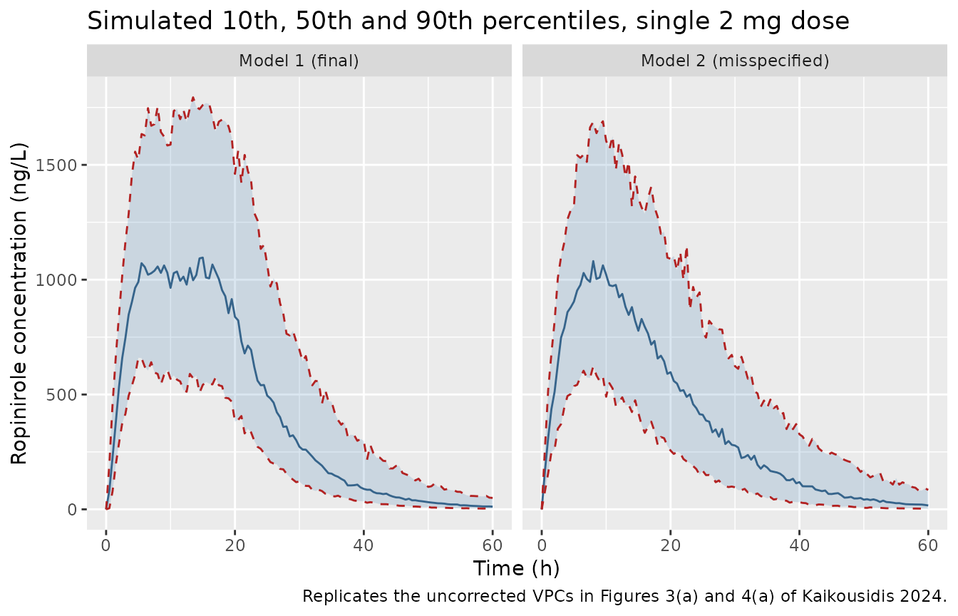
In Figure 3(a) the simulated median of Model 1 rises to roughly 1000 ng/L by about 5 h and stays near that level until about 17 h, with a second absorption arm that fills in the late plateau; in Figure 4(a) the simulated median of Model 2 peaks near 1050 ng/L at 8-10 h and then declines monotonically, missing the late plateau of the data. The maintainers read these levels from the figures. The check below is on the centre of the simulated distribution only: a mis-transcribed volume, dose or unit conversion moves it by a factor of two or more.
peak_median <- vpc |>
  group_by(treatment) |>
  summarise(peak_p50 = max(p50), t_peak_p50 = time[which.max(p50)], .groups = "drop")
knitr::kable(peak_median, digits = 1,
caption = "Peak of the simulated median concentration (ng/L) and its time (h).")| treatment | peak_p50 | t_peak_p50 |
|---|---|---|
| Model 1 (final) | 1096.1 | 15 |
| Model 2 (misspecified) | 1081.0 | 8 |
stopifnot(nrow(peak_median) == 2)
stopifnot(all(peak_median$peak_p50 > 750), all(peak_median$peak_p50 < 1400))
The paper’s point is that proportional residual error added independently at each time point makes simulated individual profiles jagged (its Figures 5 and 6, right-hand panels). Four simulated Model 1 subjects show the same effect: the smooth line is the individual prediction and the points joined by a thin line are the simulated observations at the study sampling times.
study_times <- c(0:10, 12, 14, 16, 18, 24, 36, 48, 60)
sim1 |>
  filter(id %in% 1:4) |>
  ggplot(aes(time)) +
  geom_line(aes(y = ipredSim), colour = "grey30") +
  geom_line(data = ~ filter(.x, time %in% study_times), aes(y = sim),
            colour = "firebrick", linewidth = 0.3) +
  geom_point(data = ~ filter(.x, time %in% study_times), aes(y = sim),
             colour = "firebrick", size = 1) +
  facet_wrap(~id, scales = "free_y", labeller = label_both) +
  labs(x = "Time (h)", y = "Ropinirole concentration (ng/L)",
       caption = "Compare with the uncorrected profiles in Figures 5 and 6 of Kaikousidis 2024.")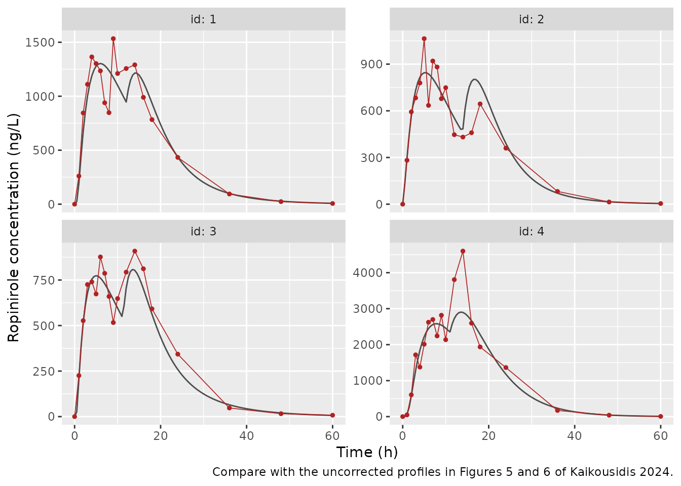
PKNCA validation
The paper reports no NCA parameters, so the NCA below characterises
the simulated profiles (individual predictions, without residual error)
and checks mass balance: with linear elimination and complete
absorption, AUC0-inf * CL / dose is 1 for every
subject.
sim_nca <- sim |>
  filter(!is.na(ipredSim)) |>
  transmute(id, time, Cc = ipredSim, treatment)
sim_nca <- bind_rows(
  sim_nca,
  sim_nca |> distinct(id, treatment) |> mutate(time = 0, Cc = 0)
) |>
  distinct(id, treatment, time, .keep_all = TRUE) |>
  arrange(id, treatment, time)

dose_df <- bind_rows(ev1, ev2) |>
  filter(evid == 1L, cmt == "depot") |>
  select(id, time, amt, treatment)

conc_obj <- PKNCA::PKNCAconc(sim_nca, Cc ~ time | treatment + id)
dose_obj <- PKNCA::PKNCAdose(dose_df, amt ~ time | treatment + id)
intervals <- data.frame(
  start = 0, end = Inf,
  cmax = TRUE, tmax = TRUE, auclast = TRUE, aucinf.obs = TRUE, half.life = TRUE
)
nca_res <- PKNCA::pk.nca(PKNCA::PKNCAdata(conc_obj, dose_obj, intervals = intervals))
summary(nca_res)
#>  start end              treatment   N      auclast        cmax
#>      0 Inf        Model 1 (final) 200 27100 [38.7] 1270 [30.2]
#>      0 Inf Model 2 (misspecified) 200 24000 [34.9] 1060 [22.1]
#>               tmax   half.life   aucinf.obs
#>  13.5 [3.50, 22.5] 7.03 [1.48] 27300 [39.1]
#>  8.50 [5.00, 13.0] 7.69 [2.01] 24300 [36.2]
#>
#> Caption: auclast, cmax, aucinf.obs: geometric mean and geometric coefficient of variation; tmax: median and range; half.life: arithmetic mean and standard deviation; N: number of subjects
cl_by_id <- sim |> distinct(id, cl)
mb <- as.data.frame(nca_res) |>
  filter(PPTESTCD == "aucinf.obs") |>
  left_join(cl_by_id, by = "id") |>
  # AUC in ng*h/L, CL in L/h, dose 2 mg = 2e6 ng.
  mutate(ratio = PPORRES * cl / 2e6)
mb_summary <- mb |>
  group_by(treatment) |>
  summarise(median_ratio = median(ratio, na.rm = TRUE),
            n = sum(!is.na(ratio)), .groups = "drop")
knitr::kable(mb_summary, digits = 3,
caption = "AUC0-inf x CL / dose by model (1 = complete mass balance).")| treatment | median_ratio | n |
|---|---|---|
| Model 1 (final) | 1 | 200 |
| Model 2 (misspecified) | 1 | 200 |
Assumptions and deviations
-
Parameter distributions. The paper does not state
the distribution of each individual parameter. The packaged models use
Monolix’s defaults: log-normal for the rate constants, times, volume and
clearance, and logit-normal for the fraction F1. The logit-normal form
is the only one consistent with Model 2’s
F1_pop = 0.9987andomega_F1 = 0.606; a log-normal F1 would exceed 1 in about half the subjects. -
Transit chain length. The relationship
nn = Mtt * Ktr - 1between the reported Mtt1 and Ktr1 and the number of transit compartments is the definition used by Monolix’s transit-compartment absorption, which the paper names but does not write out. -
Integrated transit form. Model 1 is written in an
integrated form (see “Transit absorption in Model 1”) so that subjects
with
nn < 0can be solved. It is algebraically identical to the gamma-density input, and the check above shows the two agree where both can be solved. As with any closed-form transit input, the chain term follows the most recent dose only, which is exact for the single dose studied and for repeated doses given after the previous dose has left the chain (Mtt1 is about 0.55 h). -
Dose records. Each dose must be entered twice, into
depotand intodepot2, with the full amount; the fractions F1 and 1 - F1 are applied by the models. -
Units. Concentrations are in ng/L, as in the
paper’s figures; the dose is in mg and the volume in L, so the models
multiply
central / vcby 1e6. - Machine-learning correction. The random-forest correction of the residuals, which is the subject of the paper, is not part of either model.
-
Model 2. Model 2 is packaged because the paper
reports it in full and uses it as the second case study, not because it
describes the data well; use
Kaikousidis_2024_ropinirolefor simulation. Model 2’somega_ka2(1.715) had a non-estimable RSE. - Errata. No correction notice for the paper was found on EuropePMC as of 2026-10-31.