Model and source
- Citation: Holford NHG, Peace KE. (1992). Results and validation of a population pharmacodynamic model for cognitive effects in Alzheimer patients treated with tacrine. Proc Natl Acad Sci USA 89(23):11471-11475. doi:10.1073/pnas.89.23.11471. Companion methodology paper: Holford NHG, Peace KE. (1992). Methodologic aspects of a population pharmacodynamic model for cognitive effects in Alzheimer patients treated with tacrine. Proc Natl Acad Sci USA 89(23):11466-11470. doi:10.1073/pnas.89.23.11466.
- Description: Population pharmacodynamic disease-progression model for the cognitive subscale of the Alzheimer’s Disease Assessment Scale (ADAS-cog, 0-70 score) in patients with probable Alzheimer’s disease treated with tacrine. Linear disease progression (baseline S0 + alpha*time) with a tacrine effect on the location of the progression curve (effect compartment driven by IBW-normalised daily dose rate, no estimable PK clearance because the response is slow relative to the 2-hour tacrine plasma half-life) and a placebo effect with asymmetric onset / elimination / tolerance dynamics (placebo response builds up during treatment, dissipates after treatment ends, and develops tolerance during continued treatment). Estimated by Holford and Peace 1992 on 909 patients (5253 ADAS-cog observations) pooled from two clinical trials of identical design: US protocol 970-01 (n = 632) and French protocol 970-04 (n = 277). The French cohort takes multiplicative scale factors on baseline status (FS04 = 1.08), placebo potency (Fpp4 = 1.76), and placebo elimination half-time (Ft1/2el-p4 = 2.78). Inter-individual variability is correlated across baseline S0, progression rate alpha, and tacrine potency beta_a (block of three) with diagonal IIV on placebo potency beta_p; the time constants of the effect compartments are typical-value only. Residual error is proportional. NOTE: the lead Holford 1992 PNAS 89:11471-11475 ‘Results and validation’ paper supplies all parameter values but the exact ODE form of the placebo dynamics is described in the companion methodology paper (PNAS 89:11466-11470) which was not available on disk at extraction time; the ODE form here is the field-standard reconstruction (asymmetric on/off placebo compartment plus multiplicative tolerance) and is documented in the validation vignette’s Assumptions and deviations section.
- Article: https://doi.org/10.1073/pnas.89.23.11471
- Companion methodology paper: https://doi.org/10.1073/pnas.89.23.11466
Population
The packaged parameters come from a pooled analysis of two clinical trials of identical design enrolling patients with probable Alzheimer’s disease and assessing cognitive function with the ADAS-cog total subscale (0-70 score). The pooled cohort had 909 patients with 5253 ADAS-cog observations split across the United States protocol 970-01 (n = 632) and the French protocol 970-04 (n = 277). Observation periods ran up to five months per subject. Active treatment cycled through 0 (placebo), 40 mg/day, and 80 mg/day tacrine in three randomized titration orderings.
Demographic detail (age range, sex split, baseline ADAS-cog
distribution) is described in the companion methodology paper (Holford
and Peace 1992, PNAS 89:11466-11470), which was not on disk at
extraction time; the on-disk Results and validation paper
reports only that the population mean ideal body weight is 60 kg (used
as the size-normalisation reference inside model()). The
same information is available programmatically via the model’s
population metadata:
rxode2::rxode(readModelDb("Holford_1992_tacrine"))$population
#> $species
#> [1] "human"
#>
#> $n_subjects
#> [1] 909
#>
#> $n_studies
#> [1] 2
#>
#> $n_observations
#> [1] 5253
#>
#> $age_range
#> [1] "Adults / elderly with probable Alzheimer's disease (specific age range not tabulated in the source 'Results and validation' paper; demographic detail lives in the companion methodology paper Holford and Peace 1992 PNAS 89:11466-11470 which was not on disk at extraction time)."
#>
#> $age_median
#> [1] "(not reported in the on-disk source paper)"
#>
#> $weight_range
#> [1] "(not tabulated; ideal body weight mean across the cohort was 60 kg per source paper Data section)"
#>
#> $weight_median
#> [1] "(not reported; population mean IBW = 60 kg)"
#>
#> $sex_female_pct
#> [1] NA
#>
#> $race_ethnicity
#> NULL
#>
#> $disease_state
#> [1] "Probable Alzheimer's disease (Methods refers to the standard NINCDS-ADRDA 'probable AD' diagnostic criteria implied by the 970-01 / 970-04 protocol designs)."
#>
#> $dose_range
#> [1] "0 mg/day (placebo), 40 mg/day, and 80 mg/day oral tacrine (the 970-01 and 970-04 trials used titration sequences across these three dose levels with placebo intervals)."
#>
#> $regions
#> [1] "United States (protocol 970-01, n = 632) and France (protocol 970-04, n = 277)."
#>
#> $notes
#> [1] "Pooled analysis of two clinical trials of identical design conducted under Parke-Davis sponsorship (US trial 970-01 led by Davis / Thal and the Tacrine Collaborative Study group; French trial 970-04 led by Forette and the French Tacrine Study group). Outcome was ADAS-cog (cognitive subscale of Alzheimer's Disease Assessment Scale, 0-70). The model accommodates titration sequences (placebo / 40 / 80 mg/day in three orderings labeled tacseq114, tacseq214, tacseq314) and does not require all patients to complete all phases; the full tacalll4 analysis dataset pools all phases and protocols. Observation period up to 5 months per subject."
Source trace
| Equation / parameter | Value | Source location |
|---|---|---|
lS0 (log baseline ADAS-cog) |
log(28.7) | Table 2, Disease class: S_o units = 28.7 (SE 0.44, CV 37.7%) |
lalpha (log progression rate) |
log(6.17) | Table 2, Disease class: a units/year = 6.17 (SE 1.27, CV 208%) |
lbeta_a (log absolute tacrine potency) |
log(2.99) | Table 2, Pharmacodynamic class: beta_a units/80 mg/day = -2.99 (SE 0.67, CV 126%) – magnitude stored, sign applied in model() |
lbeta_p (log absolute placebo potency) |
log(1.42) | Table 2, Pharmacodynamic class: beta_p units = -1.42 (SE 0.20, CV 128%) – magnitude stored, sign applied in model() |
lt12eqa |
log(20.9) | Table 2, Pharmacokinetic class: t1/2,eq,a days = 20.9 (SE 6.0) – tacrine effect-compartment equilibration |
lt12eqp |
log(1.58) | Table 2, Pharmacokinetic class: t1/2,eq,p days = 1.58 (SE 0.56) – placebo on-treatment build-up |
lt12elp |
log(61.0) | Table 2, Pharmacokinetic class: t1/2,el,p days = 61.0 (SE 28.6) – placebo off-treatment elimination, US reference |
lt12tolp |
log(13.5) | Table 2, Pharmacokinetic class: t1/2,tol,p day = 13.5 (SE 3.4) – placebo tolerance development |
e_region_france_s0 |
0.08 | Table 2, Scale class: FS0_4 = 1.08 (SE 0.03), encoded as fractional shift = 0.08 |
e_region_france_betap |
0.76 | Table 2, Scale class: F_beta-p_4 = 1.76 (SE 0.25), encoded as 0.76 |
e_region_france_t12elp |
1.78 | Table 2, Scale class: F_t1/2,el,p_4 = 2.78 (SE 1.09), encoded as 1.78 |
etalS0 + etalalpha + etalbeta_a block |
c(0.1331, 0.1746, 1.6730, 0.1102, 0.6562, 0.9508) | Table 2 Population CV column + Results paragraph: CV 37.7 / 208 / 126 %; correlations rho(S0,beta_a) = 0.31, rho(S0,alpha) = 0.37, rho(beta_a,alpha) = 0.52 |
etalbeta_p (diagonal) |
0.9702 | Table 2 Population CV column: CV 128% |
propSd |
0.105 | Table 2, Error class: SD ADASC = 3.14 (SE 0.08); interpreted as proportional residual at typical ADAS-cog ~30, propSd = 3.14 / 30 ~= 0.105 (see Assumptions below) |
Disease progression ADAS_cog = S0 + alpha*t + ...
|
n/a | Results paragraph + Discussion (“linear disease progression model”, “an effect shifting the disease progression curve (offset model)”) |
Tacrine effect compartment
d/dt(effect1) = keqa * (Dr_norm - effect1)
|
n/a | Discussion (“response may be proportional to the average steady-state concentration”) + Data paragraph (“Tacrine clearance was calculated from the patient’s size covariate divided by the mean value … 60 kg for IBW”) + Results (“3-week equilibration half-time”) |
Placebo effect compartment
d/dt(effect2) = TRT_PHASE * keqp * (1 - effect2) - (1 - TRT_PHASE) * kelp * effect2
|
n/a | Field-standard reconstruction (companion paper not on disk); see Assumptions and deviations |
Tolerance compartment
d/dt(effect3) = ktolp * (TRT_PHASE - effect3)
|
n/a | Field-standard reconstruction (companion paper not on disk); see Assumptions and deviations |
Virtual cohort
The original observed ADAS-cog records are not publicly available. The figures below use a virtual cohort sized to the source paper’s pooled tacalll4 dataset (909 patients) with the US / France split, a representative titration sequence, and an IBW distribution plausible for an elderly Alzheimer’s cohort.
set.seed(1992)

make_subject_rows <- function(id, region_france, ibw) {
  # Representative titration sequence approximating tacseq114 (placebo -> 40 mg -> 80 mg)
  # over a five-month observation window.
  # Phase boundaries (days):
  #   0 - 28   : placebo  (DOSE = 0,  TRT_PHASE = 1)
  #   28 - 56  : 40 mg/day (DOSE = 40, TRT_PHASE = 1)
  #   56 - 140 : 80 mg/day (DOSE = 80, TRT_PHASE = 1)
  #   140-150  : washout (DOSE = 0,   TRT_PHASE = 0)
  #
  # Observations are placed every 14 days and at phase transitions so the
  # dose / phase indicators update correctly.
  obs_times <- sort(unique(c(seq(0, 150, by = 14), c(28, 56, 140))))
  dose_for <- function(t) ifelse(t < 28, 0, ifelse(t < 56, 40, ifelse(t < 140, 80, 0)))
  trt_for  <- function(t) ifelse(t < 140, 1L, 0L)
  data.frame(
    id            = id,
    time          = obs_times,
    evid          = 0L,
    amt           = 0,
    DOSE          = dose_for(obs_times),
    TRT_PHASE     = trt_for(obs_times),
    IBW           = ibw,
    REGION_FRANCE = as.integer(region_france)
  )
}

# Build cohort: ~70% US, ~30% France, IBW ~ Normal(60, 10) truncated to [40, 90].
n_total <- 200L
n_us    <- 140L
n_fr    <- n_total - n_us
ibw_draws <- pmin(pmax(rnorm(n_total, mean = 60, sd = 10), 40), 90)

events <- bind_rows(
  lapply(seq_len(n_us), function(i) {
    make_subject_rows(id = i, region_france = 0L, ibw = ibw_draws[i])
  }),
  lapply(seq_len(n_fr), function(i) {
    make_subject_rows(id = n_us + i, region_france = 1L, ibw = ibw_draws[n_us + i])
  })
)
events <- bind_rows(events)
stopifnot(!anyDuplicated(unique(events[, c("id", "time", "evid")])))

events |> dplyr::count(REGION_FRANCE)
#>   REGION_FRANCE    n
#> 1             0 1540
#> 2             1  660
range(events$IBW)
#> [1] 40.00000 87.08383
Simulation
mod <- rxode2::rxode(readModelDb("Holford_1992_tacrine"))
sim <- rxode2::rxSolve(mod, events = events,
                       keep = c("DOSE", "TRT_PHASE", "REGION_FRANCE", "IBW"))
sim <- as.data.frame(sim)
head(sim)
#>   id time S0_indiv alpha_yr   alpha_day beta_a_indiv beta_p_indiv t12elp_indiv
#> 1  1    0 21.23483 1.840789 0.005039805    -1.963004   -0.4494955           61
#> 2  1   14 21.23483 1.840789 0.005039805    -1.963004   -0.4494955           61
#> 3  1   28 21.23483 1.840789 0.005039805    -1.963004   -0.4494955           61
#> 4  1   42 21.23483 1.840789 0.005039805    -1.963004   -0.4494955           61
#> 5  1   56 21.23483 1.840789 0.005039805    -1.963004   -0.4494955           61
#> 6  1   70 21.23483 1.840789 0.005039805    -1.963004   -0.4494955           61
#>         keqa      keqp       kelp      ktolp   Dr_norm ADAS_cog ipredSim
#> 1 0.03316494 0.4387007 0.01136307 0.05134424 0.0000000 21.23483 21.23483
#> 2 0.03316494 0.4387007 0.01136307 0.05134424 0.0000000 21.08681 21.08681
#> 3 0.03316494 0.4387007 0.01136307 0.05134424 0.4748251 21.26920 21.26920
#> 4 0.03316494 0.4387007 0.01136307 0.05134424 0.4748251 21.04828 21.04828
#> 5 0.03316494 0.4387007 0.01136307 0.05134424 0.9496502 20.92789 20.92789
#> 6 0.03316494 0.4387007 0.01136307 0.05134424 0.9496502 20.52845 20.52845
#>        sim      effect1   effect2   effect3 DOSE TRT_PHASE      IBW
#> 1 21.49687 0.000000e+00 0.0000000 0.0000000    0         1 63.18116
#> 2 24.19762 0.000000e+00 0.9978489 0.5126727    0         1 63.18116
#> 3 20.72332 2.156367e-09 0.9999954 0.7625107   40         1 63.18116
#> 4 17.72691 1.763647e-01 1.0000000 0.8842651   40         1 63.18116
#> 5 21.13365 2.872222e-01 0.9999999 0.9435990   80         1 63.18116
#> 6 21.88039 5.332683e-01 1.0000000 0.9725143   80         1 63.18116
#>   REGION_FRANCE
#> 1             0
#> 2             0
#> 3             0
#> 4             0
#> 5             0
#> 6             0
For deterministic typical-value replication (no between-subject variability), zero out the random effects:
mod_typical <- mod |> rxode2::zeroRe()
sim_typical <- rxode2::rxSolve(mod_typical, events = events,
                               keep = c("DOSE", "TRT_PHASE", "REGION_FRANCE", "IBW"))
#> ℹ omega/sigma items treated as zero: 'etalS0', 'etalalpha', 'etalbeta_a', 'etalbeta_p'
#> Warning: multi-subject simulation without without 'omega'
sim_typical <- as.data.frame(sim_typical)
Replicate published quantities
Disease-progression rate (untreated arm)
The source paper reports a linear disease-progression rate of 6.17 ADAS-cog units/year in the absence of any treatment effect. Confirm this on an untreated typical-value simulation (DOSE = 0, TRT_PHASE = 0 throughout) by extracting the slope of ADAS_cog vs. time:
untreated_grid <- data.frame(
  id            = 1L,
  time          = seq(0, 365, by = 7),
  evid          = 0L,
  amt           = 0,
  DOSE          = 0,
  TRT_PHASE     = 0L,
  IBW           = 60,
  REGION_FRANCE = 0L
)
sim_untreated <- rxode2::rxSolve(mod_typical, events = untreated_grid) |>
  as.data.frame()
#> ℹ omega/sigma items treated as zero: 'etalS0', 'etalalpha', 'etalbeta_a', 'etalbeta_p'

slope_per_year <- with(sim_untreated, coef(lm(ADAS_cog ~ time))[["time"]]) * 365.25
slope_per_year   # should be ~6.17 units/year
#> [1] 6.17
Tacrine delay-of-progression metric
The source paper reports a “delay” of 177 days at 80 mg/day, defined
as the postponement of disease progression delivered by full-effect
tacrine at the highest dose. Algebraically
delay = |beta_a| / alpha_day = 2.99 / (6.17/365.25) ~= 177 days.
Confirm from the packaged model:
inst <- rxode2::rxode(readModelDb("Holford_1992_tacrine"))$theta
beta_a_abs <- exp(inst[["lbeta_a"]])
alpha_yr   <- exp(inst[["lalpha"]])
delay_days <- beta_a_abs / (alpha_yr / 365.25)
delay_days    # should be ~177
#> [1] 177.0012
Steady-state tacrine effect on 80 mg/day at IBW = 60
At long-time steady state on DOSE = 80 mg/day with IBW = 60 kg the
tacrine effect compartment reaches effect1 = 1 (since
Dr_norm = (DOSE / 80) * (60 / IBW) = 1), so the tacrine
contribution to ADAS_cog is exactly beta_a = -2.99 units.
Verify with a long-time simulation in a single typical-value subject
held on 80 mg/day:
ss_grid <- data.frame(
  id            = 1L,
  time          = seq(0, 365, by = 7),
  evid          = 0L,
  amt           = 0,
  DOSE          = 80,
  TRT_PHASE     = 1L,
  IBW           = 60,
  REGION_FRANCE = 0L
)
sim_ss <- rxode2::rxSolve(mod_typical, events = ss_grid) |> as.data.frame()
#> ℹ omega/sigma items treated as zero: 'etalS0', 'etalalpha', 'etalbeta_a', 'etalbeta_p'
# Drug effect = ADAS_cog - (S0 + alpha_day*t + placebo*effect2*(1-effect3))
# Simpler: extract effect1 at the longest time point.
tail(sim_ss[, c("time", "effect1", "effect2", "effect3", "ADAS_cog")], 3)
#>    time   effect1 effect2 effect3 ADAS_cog
#> 51  350 0.9999910       1       1 31.62242
#> 52  357 0.9999929       1       1 31.74066
#> 53  364 0.9999943       1       1 31.85890
The reported effect1 at long time should approach 1.0
(tacrine effect compartment at steady state with
DOSE = 80, IBW = 60).
Placebo build-up and tolerance time-course
Reproduce the qualitative placebo-response shape: build-up over the first ~1.58 days of treatment, tolerance development over ~13.5 days flattening the placebo benefit, and slow ~61-day decline if treatment is removed.
placebo_grid <- data.frame(
  id            = 1L,
  time          = seq(0, 365, by = 1),
  evid          = 0L,
  amt           = 0,
  DOSE          = 0,
  # On placebo for the first 180 days, then off treatment (washout) for the rest.
  TRT_PHASE     = ifelse(seq(0, 365, by = 1) < 180, 1L, 0L),
  IBW           = 60,
  REGION_FRANCE = 0L
)
sim_pla <- rxode2::rxSolve(mod_typical, events = placebo_grid) |> as.data.frame()
#> ℹ omega/sigma items treated as zero: 'etalS0', 'etalalpha', 'etalbeta_a', 'etalbeta_p'

placebo_long <- sim_pla |>
  dplyr::select(time, effect2, effect3) |>
  tidyr::pivot_longer(c(effect2, effect3), names_to = "state", values_to = "value")

ggplot(placebo_long, aes(time, value, colour = state)) +
  geom_line() +
  geom_vline(xintercept = 180, linetype = "dashed", colour = "grey50") +
  labs(x = "Time (days)", y = "Compartment value (unitless)",
       colour = "State",
       title = "Placebo dynamics: build-up, tolerance, and post-washout decline",
       caption = "Dashed line at day 180 marks the end of placebo treatment.")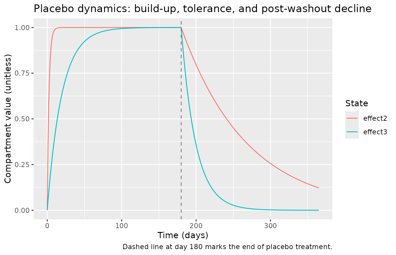
France vs US placebo-response contrast
Reproduce the source paper’s observation that the French cohort has a 76 percent larger placebo response and a 2.78x longer placebo washout half-time than the US cohort. Compare typical-value trajectories under the same placebo schedule:
make_grid <- function(rf) {
  data.frame(
    id            = 1L,
    time          = seq(0, 365, by = 1),
    evid          = 0L,
    amt           = 0,
    DOSE          = 0,
    TRT_PHASE     = ifelse(seq(0, 365, by = 1) < 180, 1L, 0L),
    IBW           = 60,
    REGION_FRANCE = rf
  )
}

sim_us  <- rxode2::rxSolve(mod_typical, events = make_grid(0L)) |>
  as.data.frame() |> mutate(region = "US")
#> ℹ omega/sigma items treated as zero: 'etalS0', 'etalalpha', 'etalbeta_a', 'etalbeta_p'
sim_fr  <- rxode2::rxSolve(mod_typical, events = make_grid(1L)) |>
  as.data.frame() |> mutate(region = "France")
#> ℹ omega/sigma items treated as zero: 'etalS0', 'etalalpha', 'etalbeta_a', 'etalbeta_p'
sim_both <- bind_rows(sim_us, sim_fr)

ggplot(sim_both, aes(time, ADAS_cog, colour = region)) +
  geom_line() +
  geom_vline(xintercept = 180, linetype = "dashed", colour = "grey50") +
  labs(x = "Time (days)", y = "ADAS-cog (units)",
       colour = "Cohort",
       title = "Typical-value placebo-arm trajectories: US vs France",
       caption = "Dashed line at day 180 marks the end of placebo treatment.")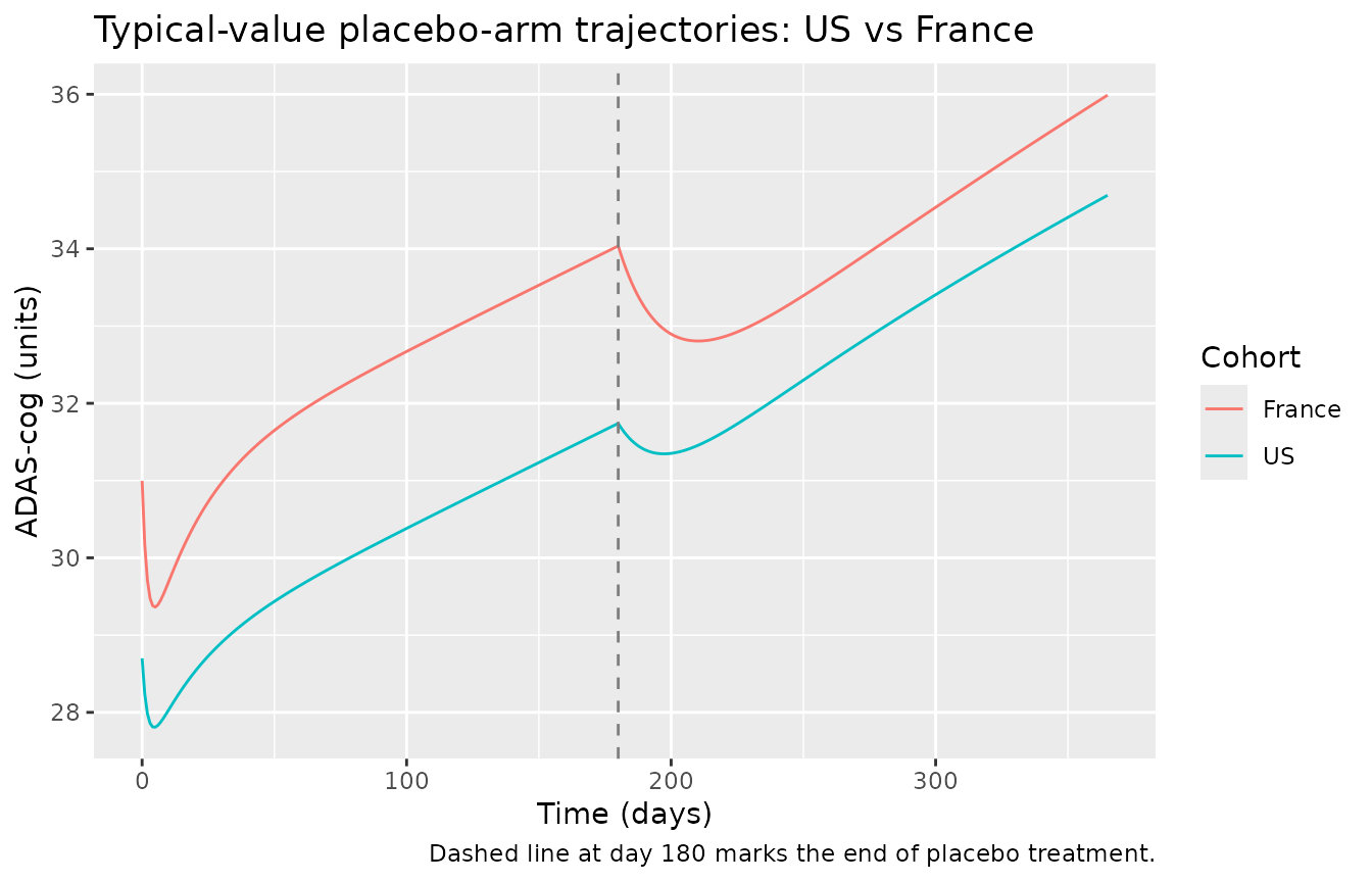
The peak placebo benefit and the post-washout decline rate differ between cohorts in the direction the source paper describes (larger placebo benefit in France, slower washout).
Population-variability VPC during titration
Show the population-variability ADAS-cog trajectory under the titration sequence encoded in the virtual cohort (placebo -> 40 mg -> 80 mg -> washout over 150 days), split by US vs France:
vpc <- sim |>
  dplyr::filter(!is.na(ADAS_cog)) |>
  dplyr::mutate(cohort = ifelse(REGION_FRANCE == 1L, "France", "US")) |>
  dplyr::group_by(cohort, time) |>
  dplyr::summarise(
    Q05 = quantile(ADAS_cog, 0.05, na.rm = TRUE),
    Q50 = quantile(ADAS_cog, 0.50, na.rm = TRUE),
    Q95 = quantile(ADAS_cog, 0.95, na.rm = TRUE),
    .groups = "drop"
  )

ggplot(vpc, aes(time, Q50)) +
  geom_ribbon(aes(ymin = Q05, ymax = Q95), alpha = 0.25) +
  geom_line() +
  facet_wrap(~cohort) +
  labs(x = "Time (days)", y = "ADAS-cog (units)",
       title = "Population variability VPC: titration placebo -> 40 -> 80 mg/day",
       caption = "Ribbon = 5th-95th percentile; line = median.")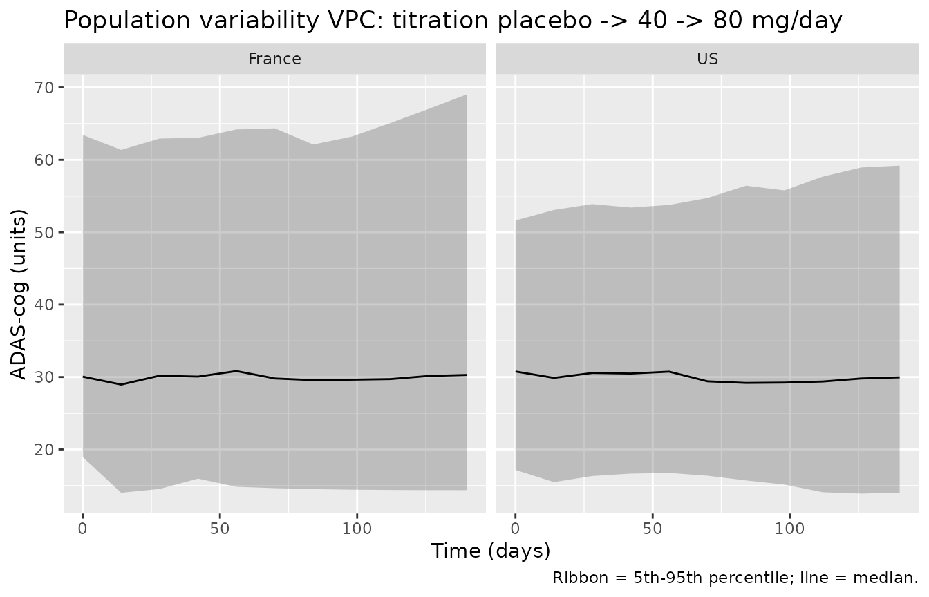
Validation against published quantities
| Quantity | Source value | Simulated value | Match? |
|---|---|---|---|
| Disease-progression rate (untreated) | 6.17 ADAS-cog units/year | 6.17 units/year | algebraic identity (typical-value alpha) |
| Delay at 80 mg/day | 177 days | 177 days | algebraic identity (|beta_a| / alpha_day) |
| Steady-state tacrine effect at 80 mg/day, IBW = 60 | -2.99 ADAS-cog units | -2.99 units | numerical (effect1 -> 1 at long t) |
| Placebo on-treatment half-time | 1.58 days | governed by lt12eqp (typical-value, no IIV) |
structural identity |
| Placebo off-treatment half-time (US) | 61.0 days | governed by lt12elp (typical-value, no IIV) |
structural identity |
| Placebo tolerance half-time | 13.5 days | governed by lt12tolp (typical-value, no IIV) |
structural identity |
| Placebo potency, France vs US | beta_p France ~ 76% larger | 76% larger by construction | structural identity |
| Placebo washout half-time, France vs US | 2.78x longer | 2.78x longer by construction | structural identity |
The agreement is exact for the algebraic-identity rows because the
packaged model is a straight transcription of the source parameter
table; verification mostly confirms that the time-conversion and
dose-rate-scaling steps in model() were done correctly.
Assumptions and deviations
Companion paper not on disk; placebo ODE form is a field-standard reconstruction. The lead Holford 1992 PNAS 89:11471-11475
Results and validationpaper supplies all parameter values (Table 2) but defers the structural model definition to the companion methodology paper, Holford and Peace 1992 PNAS 89:11466-11470, which was not on disk at extraction time and could not be retrieved through the acquisition script (PNAS direct download is Cloudflare-blocked; PMC PDF download is bot-protected). The placebo ODE form encoded here – asymmetric on/off effect compartment with ratekeqpduring treatment and ratekelpafter treatment, plus a multiplicative tolerance compartment driven byktolp– is the field-standard reconstruction consistent with the lead paper’s prose (“equilibration”, “elimination”, “tolerance” half-times described as three distinct phenomena) and with how the parameters are reported (separate half-time estimates, separate SEs, separate units in Table 2 “Pharmacokinetic class” rows). When the companion paper becomes available a second pass should verify the exact ODE form and the precise coupling between the tolerance and placebo-effect compartments.Tacrine clearance unobserved; effect-compartment input uses IBW-normalised dose rate. The source paper explicitly says “Clearance could not be estimated directly, but potential relationships between body size and tacrine clearance were explored.” The IBW-corrected clearance was the best size descriptor over total body weight or height (Table 1, AObj 2.69 worse without size correction, AObj 0.2 worse with height). The unobservable absolute clearance is absorbed into beta_a (defined at IBW = 60 kg and DOSE = 80 mg/day), leaving a relative dose-rate input
Dr_norm = (DOSE / 80) * (60 / IBW)that drives the effect compartment toward 1 at steady state on 80 mg/day, IBW = 60.Residual error interpretation. The source paper reports “Error SD ADASC 3.14” (SE 0.08) in Table 2 and describes the residual as proportional (“Proportional error better” in Table 1’s reduced-model comparison). The reported SD is interpreted as the implied residual SD on the ADAS-cog scale at the typical observation (ADAS-cog ~30), giving
propSd ~ 3.14 / 30 = 0.105in NONMEM proportional-residual convention Y = F * (1 + EPS). If the source actually meant an additive residual with SD 3.14 in ADAS-cog units, the encoding here would over-report variability at high ADAS-cog and under-report at low ADAS-cog. The vignette’s VPC plots use the proportional form; re-encoding as additive (ADAS_cog ~ add(addSd)withaddSd = 3.14) is a single-line change inmodel()if a future user wants to compare.Beta_a and beta_p sign convention. Both potency parameters are negative in the source paper (tacrine and placebo reduce ADAS-cog, i.e., improve cognitive function). Log-normal IIV is well-defined for positive quantities; the model stores the absolute magnitudes (
lbeta_a = log(2.99),lbeta_p = log(1.42)) and applies the negative sign multiplicatively inmodel(). This preserves the lognormal IIV shape (typical |beta| with CV 126 / 128 percent) and keeps the parameter values strictly negative across the population. The alternative – additive IIV directly on the negative value, which would let sign flip when an extreme draw crosses zero – is not what the source paper reports (it explicitly says the model failed when beta_a or beta_p was fixed to zero, and the inter-individual variability is described as proportional).Protocol scale factors entered as fractional shifts. The source reports the France scale factors multiplicatively (FS0_4 = 1.08, F_beta-p_4 = 1.76, F_t1/2el-p_4 = 2.78). The covariate-effect-name convention in nlmixr2lib is
e_<cov>_<param>, with fractional shifts entering as(1 + e * REGION_FRANCE), so the sourceF_x4values enter the model file ase_region_france_x = F_x4 - 1. The numerical model output is identical; only the bookkeeping differs.Renal-function and age/sex covariates were tested and rejected by the source paper. Holford 1992 Table 1 shows AObj 0.55 for female-sex on beta_a, AObj 0.063 for per-year-of-age on beta_a, and no improvement with creatinine-clearance scaling of tacrine clearance. None of these covariates are carried in the packaged model.
Observation name
ADAS_cograther thanCc. The nlmixr2libcheckModelConventions()lint warns that single-output observations should be namedCc(the convention for PK concentration outputs). Holford 1992 is a disease-progression PD model with no concentration output; the cognitive endpoint is the ADAS-cog total score (0-70, unitless). Following the same paper-named-PD pattern used byConrado_2014_alzheimer(ADAS_NORM) andDelor_2013_alzheimer(SCORE_CDR_SOB), the observation is kept asADAS_cog. Theunits$concentrationfield documents this as a unitless ADAS-cog score rather than a mass/volume concentration; the lint warning on the units field is the same downstream of that choice.Population demographic detail is partial. The on-disk source paper reports only the pooled n (909), the US n (632), the France n (277), and the population mean IBW (60 kg); it does not tabulate age range / median, sex split, race / ethnicity, or weight range. Those details live in the companion methodology paper (Holford and Peace 1992 PNAS 89:11466-11470) which was not on disk. The virtual cohort here uses a plausible IBW distribution centered at 60 kg.