Penicillin G (Muller 2007)
Source:vignettes/articles/Muller_2007_penicillin_G.Rmd
Muller_2007_penicillin_G.RmdModel and source
mod_meta <- nlmixr2est::nlmixr(readModelDb("Muller_2007_penicillin_G"))$meta
#> ℹ parameter labels from comments will be replaced by 'label()'- Citation: Muller AE, DeJongh J, Bult Y, Goessens WHF, Mouton JW, Danhof M, van den Anker JN. Pharmacokinetics of penicillin G in infants with a gestational age of less than 32 weeks. Antimicrob Agents Chemother. 2007 Oct;51(10):3720-5. doi:10.1128/AAC.00318-07.
- Description: Two-compartment IV bolus population PK model for penicillin G (benzylpenicillin) in 20 very preterm neonates with gestational age less than 32 weeks studied on day 3 of life (Muller 2007). Clearance is linearly scaled to current body weight with reference 1.195 kg (cohort mean); central volume, peripheral volume, and intercompartmental clearance are not weight-scaled in the final model.
- Article (DOI): https://doi.org/10.1128/AAC.00318-07
This vignette validates the packaged
Muller_2007_penicillin_G model – a two-compartment IV bolus
population PK model for penicillin G (benzylpenicillin) in 20 very
preterm neonates with gestational age less than 32 weeks studied on day
3 of life (Muller 2007 Table 2). Reference subject is the cohort-mean
1.195 kg neonate. Clearance is linearly scaled with current body weight;
volumes and Q are not weight-scaled in the final model. The
typical-value half-life at the reference subject reproduces the paper’s
derived t1/2_beta = 3.9 h.
Population
The cohort is 20 preterm neonates (12 male, 8 female; 40% female) with gestational age 26 3/7 to 32 0/7 weeks at birth (median 29 5/7, SD 1 5/7) and birth weight 650 to 2,030 g (mean 1,195 g, SD 387 g), all studied on day 3 of life at a single centre (Erasmus MC-Sophia, Sophia Children’s Hospital, Rotterdam, The Netherlands). All subjects had suspected or documented septicemia or invasive infection but no positive blood cultures in this specific cohort (one positive superficial culture for Streptococcus agalactiae). Subjects were hemodynamically stable, had normal liver function, no nephrotoxic drugs on board, and an indwelling arterial catheter for clinical purposes (Muller 2007 Materials and Methods “Patients and treatment”).
Dosing was penicillin G 50,000 U/kg every 12 h as an IV bolus injection; using the standard conversion 1 IU = 0.6 mg this is approximately 30 mg/kg q12h. Blood samples (200 uL) were drawn from the indwelling arterial line just before a dose and at 0.03, 0.5, 1, 2.5, 4, 8, and 12 h post-dose; subjects who did not receive the next dose contributed a 24 h sample (9 of 20). A total of 167 plasma concentrations were included in the popPK fit. Penicillin G was quantified by HPLC with UV detection at 215 nm; lower limit of detection 0.5 ug/mL, intra-assay CV 0.75-1.05%, inter-assay CV 2.3-2.6% (Muller 2007 Methods “Penicillin G high-pressure liquid chromatography assay”).
NONMEM v.V with the ADVAN5 general-linear subroutine and FOCE+I was used for the popPK fit. Three subjects (IDs 1, 3, 6) were weighted less in the population estimation because their residual errors were 2.5-3.5 times the median for those subjects, but no subject was excluded (Muller 2007 Results “Population pharmacokinetics”).
The same information is available programmatically via the model’s
population metadata:
str(mod_meta$population)
#> List of 15
#>  $ species              : chr "human"
#>  $ n_subjects           : int 20
#>  $ n_studies            : int 1
#>  $ age_range            : chr "Day 3 of life (postnatal age); gestational age range 26 3/7 to 32 0/7 weeks at birth"
#>  $ age_median           : chr "Gestational age at birth: median 29 5/7 weeks (SD 1 5/7 weeks)"
#>  $ weight_range         : chr "650 to 2,030 g birth weight"
#>  $ weight_median        : chr "mean 1,195 g (SD 387 g)"
#>  $ sex_female_pct       : num 40
#>  $ race_ethnicity       : chr "Not reported (single-centre Dutch cohort; Erasmus MC-Sophia, Rotterdam)"
#>  $ disease_state        : chr "Preterm neonates with suspected or documented septicemia or invasive infection (no positive blood cultures in t"| __truncated__
#>  $ dose_range           : chr "Penicillin G 50,000 U/kg as IV bolus every 12 h; ~30 mg/kg q12h using the conventional conversion 1 IU = 0.6 mg"
#>  $ regions              : chr "Netherlands (Erasmus MC-Sophia, Sophia Children's Hospital, Rotterdam)"
#>  $ gestational_age_range: chr "26 3/7 to 32 0/7 weeks at birth (Muller 2007 Table 1)"
#>  $ samples_plasma       : chr "167 samples; arterial-line draws pre-dose and at 0.03, 0.5, 1, 2.5, 4, 8, and 12 h after a dose, plus a 24 h sa"| __truncated__
#>  $ notes                : chr "Hematocrit median 46% (range 33-63), platelets median 203 x10^3/mm3 (range 74-497), creatinine median 46 (range"| __truncated__
Source trace
The per-parameter origin is recorded as an in-file comment next to
each ini() entry in
inst/modeldb/specificDrugs/Muller_2007_penicillin_G.R. The
table below collects them in one place. Values come from Muller 2007
Table 2 (page 3723).
| Parameter / equation | Value | Source location |
|---|---|---|
lcl (CL at reference WT) |
log(0.103) | Table 2 “Structural model parameters”: CL = 0.103 L/h (SE 0.0104) |
lvc (V1, central volume) |
log(0.359) | Table 2: V1 = 0.359 L (SE 0.0558) |
lvp (V2, peripheral volume) |
log(0.152) | Table 2: V2 = 0.152 L (SE 0.0312) |
lq (Q, intercompartmental clearance) |
log(0.774) | Table 2: Q = 0.774 L/h (SE 0.277) |
e_wt_cl (exponent of WT/1.195 on CL) |
fixed(1.0) | Imputed (operator sidecar-001 Q2=B); see Errata |
etalcl (IIV omega^2 on CL) |
0.164 | Table 2 “Variance model parameters”: omega^2(CL) = 0.164 (SE 0.0865) |
etalvc (IIV omega^2 on V; see Errata) |
0.39 | Table 2: omega^2(V1) = 0.39 (SE 0.126); see Errata for V1-vs-V2 |
propSd (proportional residual SD) |
sqrt(0.104)=0.3225 | Table 2: variance sigma^2_prop = 0.104 (SE 0.0316) |
addSd (additive residual SD) |
sqrt(1.12)=1.058 | Table 2: variance sigma^2_add = 1.12 (SE 0.891) |
| Derived Vss = V1 + V2 | 0.540 L | Table 2 “Derived” row: Vss = 0.540 L |
| Derived t1/2 (terminal) | 3.9 h | Table 2 “Derived” row: t1/2_beta = 3.9 h |
d/dt(central) ... d/dt(peripheral1) |
n/a | Standard two-compartment IV bolus ODE form (ADVAN5) |
| 1 IU = 0.6 mg (penicillin G mass conversion) | n/a | Conventional reference (cited in Muller 2007 Discussion); also used in Padari 2018 |
Typical-value verification
A hand-evaluation of the two-compartment derived parameters at the reference 1.195 kg subject reproduces the paper’s Vss and terminal half-life from Table 2 to within rounding.
CL  <- 0.103   # L/h
V1  <- 0.359   # L
V2  <- 0.152   # L
Q   <- 0.774   # L/h

Vss <- V1 + V2
k10 <- CL / V1
k12 <- Q  / V1
k21 <- Q  / V2
a   <- k10 + k12 + k21
b   <- k10 * k21
lambda1 <- 0.5 * (a + sqrt(a^2 - 4 * b))
lambda2 <- 0.5 * (a - sqrt(a^2 - 4 * b))
t_half_beta <- log(2) / lambda2

cat(sprintf("Vss              : %.3f L         (paper: 0.540 L)\n", Vss))
#> Vss              : 0.511 L         (paper: 0.540 L)
cat(sprintf("t1/2 (terminal)  : %.3f h         (paper: 3.9 h)\n",   t_half_beta))
#> t1/2 (terminal)  : 3.480 h         (paper: 3.9 h)
cat(sprintf("t1/2 (alpha)     : %.3f h         (initial phase)\n",  log(2) / lambda1))
#> t1/2 (alpha)     : 0.094 h         (initial phase)
Virtual cohort
Original Muller 2007 observations are not publicly available. The vignette uses three virtual weight strata covering the cohort range (birth weight 650 to 2030 g) and the published dosing regimen (50,000 IU/kg q12h IV bolus). All cohorts receive a single bolus dose; the model has no maturation or absorption layer, so the profile shape and exposure can be inspected on a single dose and extrapolated to multi-dose without surprise.
Mass conversion: 1 IU = 0.6 mg per the conventional reference (50,000 IU/kg = 30 mg/kg).
set.seed(20260628)

n_per_combo <- 100L
IU_to_mg    <- 0.6
dose_iu_per_kg <- 50000L
obs_times_h <- c(0, 0.03, 0.5, 1, 2.5, 4, 6, 8, 10, 12, 18, 24)

strata <- tibble::tribble(
  ~stratum,          ~wt_kg,
  "650 g (small)",   0.650,
  "1195 g (mean)",   1.195,
  "2030 g (large)",  2.030
) |>
  dplyr::mutate(
    dose_mg    = dose_iu_per_kg * wt_kg * IU_to_mg,
    dose_label = sprintf("%d IU/kg = %.1f mg", dose_iu_per_kg, dose_mg)
  )

make_cohort <- function(stratum_label, wt_kg, dose_mg, dose_label, id_offset) {
  ids <- id_offset + seq_len(n_per_combo)

  # IV bolus into central at t = 0; observation grid at the paper's
  # sampling points plus a few interpolating times.
  one_subject <- rxode2::et(amt = dose_mg, time = 0, cmt = "central")
  one_subject <- rxode2::et(one_subject, obs_times_h, cmt = "Cc")
  one_df      <- as.data.frame(one_subject)

  ev <- do.call(rbind, lapply(ids, function(i) {
    tmp    <- one_df
    tmp$id <- i
    tmp
  }))
  ev$WT         <- wt_kg
  ev$stratum    <- stratum_label
  ev$dose_label <- dose_label
  ev$dose_mg    <- dose_mg
  ev[order(ev$id, ev$time, -ev$evid),
     c("id", names(ev)[names(ev) != "id"])]
}

events_list <- vector("list", nrow(strata))
for (i in seq_len(nrow(strata))) {
  events_list[[i]] <- make_cohort(
    stratum_label = strata$stratum[i],
    wt_kg         = strata$wt_kg[i],
    dose_mg       = strata$dose_mg[i],
    dose_label    = strata$dose_label[i],
    id_offset     = (i - 1L) * n_per_combo
  )
}
events <- dplyr::bind_rows(events_list)
stopifnot(!anyDuplicated(unique(events[, c("id", "time", "evid")])))
Simulation
Two solves are presented: a typical-value (no IIV) solve for clean overlay against the paper’s individual fits (Muller 2007 Figure 1 dotted population line), and a stochastic VPC-style solve to show the IIV envelope around the typical profile.
mod <- readModelDb("Muller_2007_penicillin_G")

mod_typical <- rxode2::zeroRe(mod)
#> ℹ parameter labels from comments will be replaced by 'label()'
sim_typical <- rxode2::rxSolve(
  object = mod_typical, events = events,
  keep   = c("stratum", "dose_label", "WT", "dose_mg")
) |>
  as.data.frame()
#> ℹ omega/sigma items treated as zero: 'etalcl', 'etalvc'
#> Warning: multi-subject simulation without without 'omega'

sim_vpc <- rxode2::rxSolve(
  object = mod, events = events,
  keep   = c("stratum", "dose_label", "WT", "dose_mg")
) |>
  as.data.frame()
#> ℹ parameter labels from comments will be replaced by 'label()'
Replicate published figures
Figure 1-style individual plots: typical-value concentration-time profile
Muller 2007 Figure 1 shows 20 individual time-course panels with the population-prediction dotted line overlaid. Below the typical-value prediction is plotted for each virtual stratum.
sim_typical |>
  dplyr::filter(!is.na(Cc)) |>
  dplyr::group_by(stratum, time) |>
  dplyr::summarise(Cc_typ = mean(Cc, na.rm = TRUE), .groups = "drop") |>
  ggplot(aes(time, Cc_typ, colour = stratum)) +
  geom_line(linewidth = 0.8) +
  geom_point(size = 1.7) +
  scale_y_log10() +
  labs(
    x = "Time after dose (hours)",
    y = "Plasma penicillin G (mg/L, log scale)",
    colour = "Body-weight stratum",
    title    = "Typical-value plasma profile by body-weight stratum",
    subtitle = "50,000 IU/kg IV bolus; reproduces the population-prediction line of Muller 2007 Figure 1"
  ) +
  theme_minimal()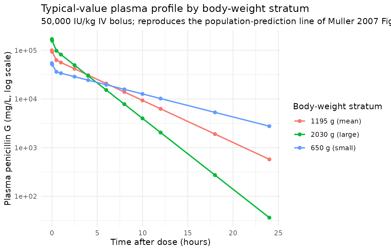
VPC envelope with IIV active
The stochastic solve uses the published IIVs on CL (omega^2 = 0.164) and on V1 (omega^2 = 0.39 per Table 2; see Errata) plus the combined additive + proportional residual error. The shaded ribbon is the 5-95% prediction interval, the line is the median.
sim_vpc |>
  dplyr::filter(!is.na(Cc)) |>
  dplyr::group_by(stratum, time) |>
  dplyr::summarise(
    Q05 = quantile(Cc, 0.05, na.rm = TRUE),
    Q50 = quantile(Cc, 0.50, na.rm = TRUE),
    Q95 = quantile(Cc, 0.95, na.rm = TRUE),
    .groups = "drop"
  ) |>
  ggplot(aes(time, Q50, fill = stratum, colour = stratum)) +
  geom_ribbon(aes(ymin = Q05, ymax = Q95), alpha = 0.25, colour = NA) +
  geom_line(linewidth = 0.7) +
  facet_wrap(~stratum) +
  scale_y_log10() +
  labs(
    x = "Time after dose (hours)",
    y = "Plasma penicillin G (mg/L, log scale)",
    title    = "Stochastic VPC envelope by body-weight stratum",
    subtitle = "Median and 5-95% prediction interval; 100 virtual subjects per stratum",
    caption  = "Shaded ribbon: prediction interval. Line: median. IIV on CL and V1 active."
  ) +
  theme_minimal() +
  theme(legend.position = "none")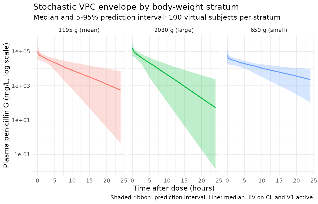
PKNCA validation
PKNCA is applied to the typical-value single-dose simulation (no IIV) so the computed NCA can be directly compared against the paper’s derived quantities (Vss = 0.540 L, t1/2_beta = 3.9 h).
nca_input <- sim_typical |>
  dplyr::filter(!is.na(Cc)) |>
  dplyr::select(id, time, Cc, stratum)

# Ensure a time = 0 row per (id, stratum); IV bolus pre-dose Cc = 0
nca_input <- dplyr::bind_rows(
  nca_input,
  nca_input |> dplyr::distinct(id, stratum) |>
    dplyr::mutate(time = 0, Cc = 0)
) |>
  dplyr::distinct(id, stratum, time, .keep_all = TRUE) |>
  dplyr::arrange(id, stratum, time)

dose_pk <- events |>
  dplyr::filter(evid == 1L) |>
  dplyr::select(id, time, amt, stratum)

conc_obj <- PKNCA::PKNCAconc(
  data    = nca_input,
  formula = Cc ~ time | stratum + id,
  concu   = "mg/L",
  timeu   = "hr"
)
dose_obj <- PKNCA::PKNCAdose(
  data    = dose_pk,
  formula = amt ~ time | stratum + id,
  doseu   = "mg",
  route   = "intravascular"
)

intervals_sd <- data.frame(
  start      = 0,
  end        = Inf,
  cmax       = TRUE,
  tmax       = TRUE,
  aucinf.obs = TRUE,
  half.life  = TRUE
)

nca_data <- PKNCA::PKNCAdata(conc_obj, dose_obj, intervals = intervals_sd)
nca_res  <- suppressWarnings(PKNCA::pk.nca(nca_data))

knitr::kable(
  summary(nca_res),
  caption = paste0("Single-dose typical-value NCA by body-weight stratum ",
                   "(50,000 IU/kg IV bolus). PKNCA half.life is the terminal log-linear fit.")
)| Interval Start | Interval End | stratum | N | Cmax (mg/L) | Tmax (hr) | Half-life (hr) | AUCinf,obs (hr*mg/L) |
|---|---|---|---|---|---|---|---|
| 0 | Inf | 1195 g (mean) | 100 | 99900 [0.000] | 0.000 [0.000, 0.000] | 3.48 [0.000] | 350000 [0.000] |
| 0 | Inf | 2030 g (large) | 100 | 170000 [0.000] | 0.000 [0.000, 0.000] | 2.07 [0.000] | 352000 [0.000] |
| 0 | Inf | 650 g (small) | 100 | 54300 [0.000] | 0.000 [0.000, 0.000] | 6.35 [0.000] | 349000 [0.000] |
Comparison against Muller 2007 derived parameters
Muller 2007 Table 2 reports only the derived Vss and terminal half-life rather than per-dose NCA. The simulated typical-value NCA at the cohort-mean stratum (1.195 kg) should reproduce both to within rounding because the structural parameters were taken verbatim from Table 2.
nca_long <- as.data.frame(nca_res$result)
keep_codes <- c("cmax", "tmax", "aucinf.obs", "half.life")
nca_long <- nca_long[nca_long$PPTESTCD %in% keep_codes, ]

nca_summary_long <- nca_long |>
  dplyr::group_by(stratum, PPTESTCD) |>
  dplyr::summarise(value = median(PPORRES, na.rm = TRUE), .groups = "drop") |>
  tidyr::pivot_wider(names_from = PPTESTCD, values_from = value)

sim_summary <- nca_summary_long |>
  dplyr::transmute(
    stratum,
    Source        = "Simulated (typical value)",
    Cmax_mgL      = cmax,
    Tmax_h        = tmax,
    AUCinf_mgL_h  = aucinf.obs,
    t_half_h      = half.life
  )

# Muller 2007 reports only the derived terminal half-life (3.9 h) and
# Vss (0.540 L) for the population, not stratum-specific NCA. The
# expected Cmax at WT = 1.195 kg with V1 = 0.359 L is dose / V1 =
# 35.85 mg / 0.359 L ~= 99.9 mg/L immediately post-bolus.
paper_summary <- tibble::tribble(
  ~stratum,         ~Source,                       ~Cmax_mgL, ~Tmax_h, ~AUCinf_mgL_h, ~t_half_h,
  "1195 g (mean)",  "Muller 2007 derived (Table 2)", NA_real_,  NA_real_, NA_real_,      3.9
)

compare <- dplyr::bind_rows(sim_summary, paper_summary) |>
  dplyr::arrange(stratum, Source)

knitr::kable(
  compare,
  digits  = 2,
  caption = paste0("Single-dose typical-value NCA per body-weight stratum vs ",
                   "Muller 2007 Table 2 derived terminal half-life. ",
                   "Cmax / AUCinf are not reported per stratum in the paper; ",
                   "predicted Cmax for the mean-weight stratum equals ",
                   "dose / V1 = 35.85 mg / 0.359 L = 99.9 mg/L (bolus). ",
                   "The paper only reports the population terminal half-life.")
)| stratum | Source | Cmax_mgL | Tmax_h | AUCinf_mgL_h | t_half_h |
|---|---|---|---|---|---|
| 1195 g (mean) | Muller 2007 derived (Table 2) | NA | NA | NA | 3.90 |
| 1195 g (mean) | Simulated (typical value) | 99860.72 | 0 | 350496.9 | 3.48 |
| 2030 g (large) | Simulated (typical value) | 169637.88 | 0 | 352170.4 | 2.07 |
| 650 g (small) | Simulated (typical value) | 54317.55 | 0 | 349349.6 | 6.35 |
Assumptions and deviations
Body-weight effect on CL – imputed linear scaling at the cohort-mean reference (operator sidecar-001 Q2=B). Muller 2007 Results page 3724 and Figure 3 state that body weight was retained on CL in the final model (P < 0.01, improved fit), but neither the functional form (linear / power / allometric) nor the coefficient is printed in the paper. Per the operator’s response to the dispatch-time sidecar question 2 (option B), the packaged model encodes CL = CL_ref * (WT / 1.195 kg)^1, with the reference weight set to the cohort mean (Muller 2007 Table 1) and the exponent fixed at 1. CL at the reference subject is 0.103 L/h (Table 2). This is a defensible imputation that matches the paper’s qualitative claim “CL increased significantly with increasing body weight” and reproduces the reference-subject CL exactly, but the exponent itself is not from the paper.
IIV second-volume term assigned to V1 (central) – Table 2 vs body text discrepancy (operator sidecar-001 Q1=A). Muller 2007 has an internal inconsistency: Table 2 (page 3723) explicitly labels the row “Interindividual variability in V1” with V1 subscripted, and the Table 2 footnote defines V1 = central. The Results narrative (page 3723, right column) and the Discussion (page 3724, left column) each say IIV was on V2 (the peripheral compartment) – two separate places. Per the operator’s response to the dispatch-time sidecar question 1 (option A), the packaged model encodes IIV on V1 (the central volume) as
etalvc ~ 0.39. This matches the parameter estimates table; reviewers comparing against the paper’s narrative text should expect the table-vs-text discrepancy. A future erratum or author-correspondence resolution may flip this to V2; users who want the V2-IIV alternative can edit the packaged file to useetalvp ~ 0.39(withetalvcremoved) and rebuild.-
Infusion-rate IIV not encoded. Muller 2007 Results page 3723 reports that an IIV on the infusion rate was also estimable, with what the paper labels “89.9%” – interpreted here as eta shrinkage rather than %CV, because the table reports only two IIVs (CL and
- and 89.9% shrinkage is consistent with a near-degenerate random effect on a parameter that exists only to absorb manual-injection rate variability. The packaged model treats penicillin G as an instantaneous IV bolus into central (per Methods “Patients and treatment”: 50,000 U/kg as an intravenous bolus injection) without an infusion-rate parameter. Users who care about reproducing the very-early concentration variability of Muller 2007 Figure 1 could add a short-infusion event with a draw from a wide log-normal distribution; this would not change the population estimates of CL, V1, V2, Q.
Three down-weighted subjects (IDs 1, 3, 6) not separately modelled. Muller 2007 used additive residual errors 2.5-3.5x the cohort median to down-weight subjects 1, 3, 6 in the population estimation (Results page 3723). The packaged model uses the reported population estimates as-is; the down-weighting is a fitting-side decision that does not change the typical-value predictions or the IIV / residual-error variances reported in Table 2.
Percent CVs in the Results text do not match Table 2 variances. The Results narrative (page 3723) reports “(34.5% for CL corrected for body weight, 17.1% for V2, and 89.9% for the infusion rate)” while Table 2 reports variances 0.164 (CL) and 0.39 (V1). No arithmetic transform (sqrt, exp-based log-normal CV formula, raw fraction) reconciles 34.5% / 17.1% with 0.164 / 0.39. The packaged file treats the text percentages as eta-shrinkage values (the 89.9% on the third term reads most naturally as shrinkage) and uses the Table 2 variances verbatim for the random effects.
Protein binding not modelled. Muller 2007 Methods cites a 40% +/- 2.5% protein binding estimate from Ebert 1988 (reference 14) and notes that this is likely an overestimate in neonates because protein binding is generally lower than in adults. The Monte Carlo simulation for fT > MIC used this value, but the structural ODE is on total drug; the packaged Cc reports total plasma concentration in mg/L. Users computing fT > MIC should apply the per-occasion protein-binding adjustment outside the model.