Vancomycin in critically ill children (Downes 2023)
Source:vignettes/articles/Downes_2023_vancomycin.Rmd
Downes_2023_vancomycin.RmdModel and source
Downes 2023 developed three nonparametric population PK models for intravenous vancomycin in critically ill children, all sharing the same two-compartment structure and allometric body-weight scaling but differing in which renal-function covariate enters clearance. All three are packaged separately because the paper carries all three forward into its Bayesian AUC-estimation evaluation and reports a complete parameter set for each.
MODELS <- c(
  Full     = "Downes_2023_vancomycin_full",
  Hoek     = "Downes_2023_vancomycin_hoek",
  Schwartz = "Downes_2023_vancomycin_schwartz"
)
uis <- lapply(MODELS, function(n) rxode2::rxode(readModelDb(n)))
#> ℹ parameter labels from comments will be replaced by 'label()'- Citation: Downes KJ, Zuppa AF, Sharova A, Neely MN. Optimizing Vancomycin Therapy in Critically Ill Children: A Population Pharmacokinetics Study to Inform Vancomycin Area under the Curve Estimation Using Novel Biomarkers. Pharmaceutics. 2023;15(5):1336. doi:10.3390/pharmaceutics15051336
- Article: https://doi.org/10.3390/pharmaceutics15051336
- Supplement (Tables S1-S5, Figures S1-S2): https://www.mdpi.com/article/10.3390/pharmaceutics15051336/s1
| Model file | Covariate on clearance | Role in the paper |
|---|---|---|
Downes_2023_vancomycin_full |
cystatin-C eGFR (Hoek) and urinary NGAL / urine creatinine | Full model; the paper’s biomarker hypothesis |
Downes_2023_vancomycin_hoek |
cystatin-C eGFR (Hoek) only | Reduced model the authors recommend clinically |
Downes_2023_vancomycin_schwartz |
creatinine eGFR (bedside Schwartz) only | Most parsimonious; covariate universally available |
The paper’s conclusion is a negative result worth stating plainly: adding the urinary kidney-injury biomarker improved the fit substantially, but did not improve Bayesian AUC24 estimation over either reduced model, and made it markedly worse under limited sampling (Table 3).
Population
The models were estimated from the 30-subject model training group of a prospective observational study run in the PICU at the Children’s Hospital of Philadelphia between August 2018 and July 2021 (Downes 2023 Table 1). Children aged 1-17 years receiving intermittent IV vancomycin for a suspected infection were eligible; renal replacement therapy, plasmapheresis and ECMO were exclusions, and infants under 1 year were excluded deliberately because cystatin C is confounded by renal maturation over the first year of life. The authors state explicitly that the models must not be applied to infants.
Training-group medians at PK sampling: age 9.8 years (IQR 3.8-11.2), weight 25.9 kg (IQR 13.9-41.8), 37% female, serum creatinine 0.30 mg/dL (IQR 0.20-0.48), eGFR-Hoek 143 mL/min/1.73 m^2 (IQR 110-197), eGFR-Schwartz 164 (IQR 114-222), vancomycin dose 13.2 mg/kg (IQR 10.0-14.8), vasopressors in 47%. Half the training group met the paper’s augmented-renal-clearance definition of eGFR > 130 mL/min/1.73 m^2, so the cohort skews supranormal and the models carry very little information about renal impairment. The 30 subjects contributed 150 concentrations (3.9-67.8 ug/mL, 2 below the 3.0 ug/mL LLOQ).
A separate 20-subject model testing group was held out and used only to evaluate Bayesian AUC24 estimation (Table 3). Its covariate distribution is the basis of the virtual cohort below, because Table 3 is the only published table this vignette can compare simulated exposures against.
str(uis[["Full"]]$population, max.level = 1, give.attr = FALSE)
#> List of 15
#>  $ species         : chr "human"
#>  $ n_subjects      : int 30
#>  $ n_studies       : int 1
#>  $ n_sites         : int 1
#>  $ n_concentrations: int 150
#>  $ age_range       : chr "1-17 years (eligibility); Table 1 training-group median 9.8 years, IQR 3.8-11.2"
#>  $ age_median      : chr "9.8 years (IQR 3.8-11.2)"
#>  $ weight_range    : chr "IQR 13.9-41.8 kg (full range not reported)"
#>  $ weight_median   : chr "25.9 kg (IQR 13.9-41.8)"
#>  $ sex_female_pct  : num 37
#>  $ disease_state   : chr "Critically ill children in a single quaternary-care PICU receiving intermittent IV vancomycin for a suspected i"| __truncated__
#>  $ dose_range      : chr "Clinician-chosen intermittent IV regimens; typical initial dosages 10-15 mg/kg/dose every 6-8 h. Table 1 traini"| __truncated__
#>  $ regions         : chr "United States (Children's Hospital of Philadelphia, Philadelphia PA)"
#>  $ renal_function  : chr "eGFR-Hoek median 143 mL/min/1.73 m^2 (IQR 110-197) and eGFR-Schwartz median 164 (IQR 114-222) at PK sampling; s"| __truncated__
#>  $ notes           : chr "Prospective observational study conducted August 2018 to July 2021. 50 evaluable subjects were split into a 30-"| __truncated__
Source trace
Per-parameter origin is recorded as an in-file comment beside each
ini() entry. Collected here for review. Table 2 (main
paper) reports the full model; Table S4 (supplement) reports all three
side by side.
| Parameter | Full | Hoek | Schwartz | Source |
|---|---|---|---|---|
lcl (CL0, L/h) |
3.31 | 2.61 | 2.82 | Table 2 / Table S4, row CL0 |
lvc (VC0, L) |
3.50 | 5.09 | 5.09 | Table 2 / Table S4, row VC0 |
lq (Q0, L/h) |
7.09 | 6.18 | 6.27 | Table 2 / Table S4, row Q0 |
lvp (VP0, L) |
7.75 | 8.30 | 7.33 | Table 2 / Table S4, row VP0 |
e_wt_cl_q |
0.75 (fixed) | 0.75 (fixed) | 0.75 (fixed) | Methods 2.3; Table 2 rows CLWT / QWT print no CV% |
e_wt_vc_vp |
1 (fixed) | 1 (fixed) | 1 (fixed) | Methods 2.3; Table 2 rows VC-WT / VP-WT print no CV% |
e_crcl_cl |
0.85 | 1.00 | 0.32 | Table 2 row CLHOEK / Table S4 row CLEGFR |
e_ungalcr_cl |
0.94 | n/a | n/a | Table 2 row CLNGAL |
| Reference weight | 27 kg | 27 kg | 27 kg | Methods 2.3 and the Table S4 equations |
| Reference eGFR | 134 | 134 | 156 | Table S4 equations (Hoek 134, Schwartz 156) |
| IIV (CV%) | 39.5 / 49.2 / 32.6 / 39.0 / 62.8 / 10.9 | not reported | not reported | Table 2 CV% column |
addSd = 1.5, propSd = 0.1 |
fixed | fixed | fixed | Methods 2.3 assay polynomial SD = C0 + C1 * C
|
Clearance equation (Table 2 footnote, reproduced in Table S4):
CL = CL0 * (WT/27)^CLWT * (HOEK/134)^CLHOEK * (CLNGAL)^LNGALwith LNGAL the natural logarithm of
uNGAL/uCr. Note that CLNGAL is the
base of an exponential, not a power exponent, and that
the term carries no reference normalization – so CL0 is the
clearance at UNGALCR = 1 ng/mg, which is far below every
observed value. That makes the full model’s CL0
non-comparable with the two reduced models’ CL0 on its own;
see the concordance check below, which is what pins this reading.
Verification 1: transcription against a hand-typed closed form
The strongest available check on the packaged files is exact rather
than statistical. A two-compartment model receiving a constant-rate
infusion at steady state has a closed-form bi-exponential solution. The
function below is written only from the paper’s printed
constants, independently of the model files, so any
transcription error in inst/modeldb/ makes it disagree.
# Steady-state concentration for a 2-compartment model, constant-rate infusion
# of `dose` over `tinf`, repeated every `tau`. Derived from first principles;
# no model-file quantity is used.
cf_ss <- function(t, dose, tinf, tau, cl, vc, q, vp) {
  k10 <- cl / vc; k12 <- q / vc; k21 <- q / vp
  b <- k10 + k12 + k21
  d <- sqrt(b * b - 4 * k10 * k21)
  lam <- c((b + d) / 2, (b - d) / 2)                       # alpha, beta
  A <- c((k21 - lam[1]) / (vc * (lam[2] - lam[1])),
         (k21 - lam[2]) / (vc * (lam[1] - lam[2])))
  r0 <- dose / tinf
  out <- numeric(length(t))
  for (i in 1:2) {
    ai <- A[i] / lam[i]; L <- lam[i]; during <- t <= tinf
    out[during] <- out[during] + r0 * ai *
      ((1 - exp(-L * t[during])) + (1 - exp(-L * tinf)) *
         exp(-L * (t[during] + tau - tinf)) / (1 - exp(-L * tau)))
    out[!during] <- out[!during] + r0 * ai * (1 - exp(-L * tinf)) *
      exp(-L * (t[!during] - tinf)) / (1 - exp(-L * tau))
  }
  out
}

# Parameter equations typed directly from Downes 2023 Table 2 / Table S4.
hand_params <- list(
  Full = function(WT, CRCL, UNGALCR) list(
    cl = 3.31 * (WT / 27)^0.75 * (CRCL / 134)^0.85 * 0.94^log(UNGALCR),
    vc = 3.50 * (WT / 27), q = 7.09 * (WT / 27)^0.75, vp = 7.75 * (WT / 27)),
  Hoek = function(WT, CRCL, UNGALCR) list(
    cl = 2.61 * (WT / 27)^0.75 * (CRCL / 134)^1.00,
    vc = 5.09 * (WT / 27), q = 6.18 * (WT / 27)^0.75, vp = 8.30 * (WT / 27)),
  Schwartz = function(WT, CRCL, UNGALCR) list(
    cl = 2.82 * (WT / 27)^0.75 * (CRCL / 156)^0.32,
    vc = 5.09 * (WT / 27), q = 6.27 * (WT / 27)^0.75, vp = 7.33 * (WT / 27))
)
TAU <- 8; TINF <- 1
gate_grid <- sort(unique(c(seq(0, TAU, by = 0.02), TINF)))

solve_typical <- function(nm, ev) {
  m <- readModelDb(nm)
  # zeroRe() is only meaningful when the model actually declares etas; the two
  # reduced models declare none (Table S4 reports no CV%).
  if (any(!is.na(rxode2::rxode(m)$iniDf$neta1))) m <- rxode2::zeroRe(m)
  # Tight tolerances: the closed-form gate below is held to 1e-6; the ODE at
  # default tolerances lands at 1-2e-6, at rtol 1e-10 far below.
  as.data.frame(rxode2::rxSolve(m, events = ev, returnType = "data.frame", rtol = 1e-10, atol = 1e-12,
                                # steady-state searches for long-half-life subjects exceed the default step budget
                                maxsteps = 1e6))
}

one_subject_ss <- function(dose, covs, times) {
  ev <- rbind(
    data.frame(time = 0, amt = dose, evid = 1L, cmt = "central",
               ii = TAU, ss = 1L, dur = TINF),
    data.frame(time = times, amt = NA_real_, evid = 0L, cmt = "central",
               ii = 0, ss = 0L, dur = 0)
  )
  ev$id <- 1L
  for (nm in names(covs)) ev[[nm]] <- covs[[nm]]
  ev
}

# Two covariate points per model. The reference point checks the table values
# themselves; the second point additionally exercises every exponent and every
# reference constant (all of which cancel at the reference point).
gate_points <- tibble::tribble(
  ~point,              ~WT,   ~HOEK, ~SCHWARTZ, ~UNGALCR,
  "reference subject", 27,    134,   156,       1,
  "median test subject", 37.6, 130,  156,       35.3
)

gate <- lapply(seq_len(nrow(gate_points)), function(i) {
  gp <- gate_points[i, ]
  lapply(names(MODELS), function(lab) {
    crcl <- if (lab == "Schwartz") gp$SCHWARTZ else gp$HOEK
    covs <- list(WT = gp$WT, CRCL = crcl)
    if (lab == "Full") covs$UNGALCR <- gp$UNGALCR
    dose <- 15 * gp$WT
    s <- solve_typical(MODELS[[lab]], one_subject_ss(dose, covs, gate_grid))
    p <- hand_params[[lab]](gp$WT, crcl, gp$UNGALCR)
    ref <- cf_ss(s$time, dose, TINF, TAU, p$cl, p$vc, p$q, p$vp)
    tibble(point = gp$point, model = lab, CL = p$cl,
           max_rel_err = max(abs(s$Cc - ref) / ref))
  }) |> bind_rows()
}) |> bind_rows()
#> ℹ parameter labels from comments will be replaced by 'label()'
#> ℹ parameter labels from comments will be replaced by 'label()'
#> ℹ omega/sigma items treated as zero: 'etalcl', 'etalvc', 'etalq', 'etalvp', 'etae_crcl_cl', 'etae_ungalcr_cl'
#> ℹ parameter labels from comments will be replaced by 'label()'
#> ℹ parameter labels from comments will be replaced by 'label()'
#> ℹ omega/sigma items treated as zero: 'etalcl', 'etalvc', 'etalq', 'etalvp', 'etae_crcl_cl', 'etae_ungalcr_cl'

gate |>
  mutate(`Max relative error` = format(max_rel_err, digits = 2, scientific = TRUE)) |>
  select(Point = point, Model = model, `CL (L/h)` = CL, `Max relative error`) |>
  knitr::kable(digits = 3,
caption = "Packaged model vs. an independent closed form built from the printed constants.")| Point | Model | CL (L/h) | Max relative error |
|---|---|---|---|
| reference subject | Full | 3.310 | 8.7e-10 |
| reference subject | Hoek | 2.610 | 1.2e-07 |
| reference subject | Schwartz | 2.820 | 4.0e-08 |
| median test subject | Full | 3.317 | 1.5e-07 |
| median test subject | Hoek | 3.246 | 1.9e-07 |
| median test subject | Schwartz | 3.615 | 1.5e-07 |
# Pure numerical error between a solve and its own closed form: a tight bound is
# correct here and is NOT a cohort-derived quantity, so it is machine-stable.
stopifnot(nrow(gate) == 6, all(is.finite(gate$max_rel_err)),
          max(gate$max_rel_err) < 1e-6)
Agreement is at solver tolerance, so every structural parameter, every allometric exponent, both eGFR reference constants and the unnormalized NGAL term are transcribed as printed.
Verification 2: cross-model concordance pins the NGAL reading
The NGAL term is the one place the paper’s notation is genuinely easy
to misread: (CLNGAL)^LNGAL looks like a covariate power
term, but it has no reference normalization, so dropping it entirely (or
normalizing it to the cohort median) changes CL0’s meaning.
Because the three models were fitted independently to the same
30 subjects, they must predict nearly the same clearance for
the same child. That turns into a falsification test.
med <- list(WT = 37.6, HOEK = 130, SCHWARTZ = 156, UNGALCR = 35.3)
cl_of <- function(lab, drop_ngal = FALSE) {
  crcl <- if (lab == "Schwartz") med$SCHWARTZ else med$HOEK
  p <- hand_params[[lab]](med$WT, crcl, if (drop_ngal) 1 else med$UNGALCR)
  p$cl
}
spread <- function(x) 100 * (max(x) / min(x) - 1)

cl_correct <- vapply(names(MODELS), cl_of, numeric(1))
cl_dropped <- c(Full = cl_of("Full", drop_ngal = TRUE),
                cl_correct[c("Hoek", "Schwartz")])

conc_tab <- tibble(
  Reading = c("As printed (NGAL term retained, unnormalized)",
              "Misreading: NGAL term dropped"),
  `Full (L/h)`     = c(cl_correct[["Full"]],     cl_dropped[["Full"]]),
  `Hoek (L/h)`     = c(cl_correct[["Hoek"]],     cl_dropped[["Hoek"]]),
  `Schwartz (L/h)` = c(cl_correct[["Schwartz"]], cl_dropped[["Schwartz"]]),
  `Spread (%)`     = c(spread(cl_correct), spread(cl_dropped))
)
knitr::kable(conc_tab, digits = 2,
caption = "Typical clearance for the median testing-group child under two readings of the NGAL term.")| Reading | Full (L/h) | Hoek (L/h) | Schwartz (L/h) | Spread (%) |
|---|---|---|---|---|
| As printed (NGAL term retained, unnormalized) | 3.32 | 3.25 | 3.62 | 11.37 |
| Misreading: NGAL term dropped | 4.14 | 3.25 | 3.62 | 27.40 |
# Deterministic (fixed covariate values, no simulated cohort), so a tight bound
# is safe. The as-printed reading gives ~11%; the misreading gives ~27%.
stopifnot(spread(cl_correct) < 20, spread(cl_dropped) > 20)
Retaining the term as printed brings three independently estimated models to within ~11% of each other; dropping it pushes the full model ~27% away from its siblings. The packaged reading is the one that reconciles them.
Virtual cohort
Individual data are not public. The cohort below reproduces the testing group’s published covariate quantiles (Table 1 and Table S3), because Table 3 – the only published exposure table – is computed on that group. Each covariate is drawn log-normally with its median as the location and its published interquartile range setting the scale, then clipped to the reported observed range where one is given.
# set.seed() seeds R's RNG only. rxode2's own streams are partitioned per solver
# thread, so a machine with a different thread count draws a different cohort.
# Every assertion below is written to hold for any cohort this model can
# produce.
set.seed(20230425)

N <- 200L  # per arm; validation cohorts are capped at 200
lnq <- function(n, med, q1, q3) {
  stats::rlnorm(n, meanlog = log(med), sdlog = log(q3 / q1) / (2 * stats::qnorm(0.75)))
}

subj <- tibble(
  subject  = seq_len(N),
  # Table 1, testing group, at start of vancomycin / at PK sampling
  WT       = pmin(pmax(lnq(N, 37.6, 14.4, 57.5), 8), 110),
  HOEK     = lnq(N, 130, 96, 156),
  SCHWARTZ = lnq(N, 156, 134, 184),
  # Table S3 testing group median (IQR); Discussion gives the range 7.8-10034
  UNGALCR  = pmin(pmax(lnq(N, 35.3, 18.7, 62.1), 7.8), 10034)
)

# The same 200 children are used for every arm (common random numbers), so
# arm-to-arm differences are model differences, not cohort differences.
obs_grid <- sort(unique(c(seq(0, 24, by = 0.25), 1, 9, 17)))
DOSE_MGKG <- 15  # Table 1: testing-group median 15.0 mg/kg (IQR 14.5-15.7)

make_arm <- function(arm, crcl_col, id_offset) {
  s <- subj |>
    mutate(id = id_offset + subject, arm = arm, CRCL = .data[[crcl_col]],
           dose = DOSE_MGKG * WT)
  dosing <- s |>
    transmute(id, subject, arm, WT, CRCL, UNGALCR, dose,
              time = 0, amt = dose, evid = 1L, cmt = "central",
              ii = TAU, ss = 1L, dur = TINF) |>
    # ss = 1 on the first record establishes steady state; the two further
    # doses carry it through the full 24 h window (tau = 8 divides 24, so
    # AUC0-24 is phase-independent).
    tidyr::expand_grid(dose_time = c(0, 8, 16)) |>
    mutate(time = dose_time, ii = ifelse(dose_time == 0, TAU, 0),
           ss = ifelse(dose_time == 0, 1L, 0L)) |>
    select(-dose_time)
  obs <- s |>
    select(id, subject, arm, WT, CRCL, UNGALCR, dose) |>
    tidyr::expand_grid(time = obs_grid) |>
    mutate(amt = NA_real_, evid = 0L, cmt = "central", ii = 0, ss = 0L, dur = 0)
  bind_rows(dosing, obs) |> arrange(id, time, desc(evid))
}

events <- bind_rows(
  make_arm("Full",     "HOEK",     0L),
  make_arm("Hoek",     "HOEK",     1000L),
  make_arm("Schwartz", "SCHWARTZ", 2000L),
  make_arm("Full (with IIV)", "HOEK", 3000L)
)
# Duplicate ids across arms would silently merge subjects and sum their doses.
stopifnot(!anyDuplicated(unique(events[, c("id", "time", "evid")])))
Simulation
Three arms are typical-value predictions (the two reduced models declare no IIV at all, so a typical-value comparison is the only like-for-like one). A fourth arm carries the full model’s reported variability, to show the width of the nonparametric density.
KEEP <- c("arm", "subject", "WT", "CRCL", "UNGALCR", "dose")

sim <- bind_rows(
  lapply(c("Full", "Hoek", "Schwartz"), function(a)
    solve_typical(MODELS[[a]], events |> filter(arm == a)) ),
  # Full model WITH its reported CV% on all six estimated parameters.
  as.data.frame(rxode2::rxSolve(
    readModelDb(MODELS[["Full"]]),
    events = events |> filter(arm == "Full (with IIV)"),
    keep = KEEP, returnType = "data.frame",
    # steady-state searches for long-half-life subjects exceed the default step budget
    maxsteps = 1e6))
)
#> ℹ parameter labels from comments will be replaced by 'label()'
#> ℹ parameter labels from comments will be replaced by 'label()'
#> ℹ omega/sigma items treated as zero: 'etalcl', 'etalvc', 'etalq', 'etalvp', 'etae_crcl_cl', 'etae_ungalcr_cl'
#> Warning: multi-subject simulation without without 'omega'
#> Warning: multi-subject simulation without without 'omega'
#> Warning: multi-subject simulation without without 'omega'
#> ℹ parameter labels from comments will be replaced by 'label()'
# The three typical arms lose `keep` columns through zeroRe(); reattach by id.
sim <- sim |>
  select(-any_of(KEEP)) |>
  left_join(events |> filter(evid == 1L, time == 0) |>
              select(id, all_of(KEEP)), by = "id")

stopifnot(nrow(sim) > 0, !anyNA(sim$Cc), all(sim$Cc >= 0))
Concentration-time profiles
Downes 2023 publishes no typical-value profile figure. Figure 2 is an observed-versus-individual-predicted scatter and Figure S1 plots the raw observations, and neither can be reproduced without the subject-level data, which the paper makes available only on request. The panels below therefore show what the packaged models predict rather than replicating a published figure.
sim |>
  group_by(arm, time) |>
  summarise(Q05 = quantile(Cc, 0.05), Q50 = median(Cc), Q95 = quantile(Cc, 0.95),
            .groups = "drop") |>
  mutate(arm = factor(arm, levels = c("Full", "Hoek", "Schwartz", "Full (with IIV)"))) |>
  ggplot(aes(time, Q50)) +
  geom_ribbon(aes(ymin = Q05, ymax = Q95), alpha = 0.25, fill = "steelblue") +
  geom_line(linewidth = 0.7) +
  geom_hline(yintercept = c(5, 15), linetype = "dashed", colour = "grey40") +
  facet_wrap(~arm, nrow = 1) +
  labs(x = "Time within the steady-state day (h)", y = "Vancomycin (ug/mL)",
       caption = paste("Median and 5th-95th percentile across 200 virtual children at",
                       "15 mg/kg q8h (1 h infusion). Dashed lines: the 5-15 ug/mL",
                       "trough range Downes 2023 used for TDM (Methods 2.2).",
                       "The first three panels vary only by covariates; the fourth",
                       "adds the full model's reported CV%."))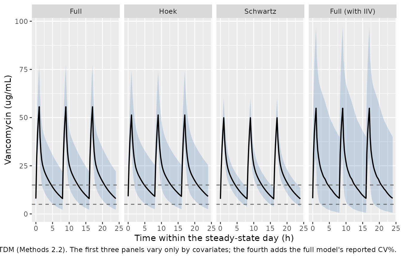
PKNCA validation
tau = 8 h divides 24, so AUC0-24 over a steady-state day
is phase-independent and PKNCA can compute it directly over the 0-24 h
window.
# Only `!is.na(Cc)`: a `time > 0` or `Cc > 0` filter would drop the time-zero
# record PKNCA needs to anchor the interval. At steady state that record is the
# trough, not zero, so it must NOT be overwritten with Cc = 0 either.
sim_nca <- sim |>
  filter(!is.na(Cc)) |>
  select(id, time, Cc, arm)
stopifnot(nrow(sim_nca) > 0,
          all(tapply(sim_nca$time, sim_nca$id, min) == 0))  # time-zero present

conc_obj <- PKNCA::PKNCAconc(sim_nca, Cc ~ time | arm + id,
                             concu = "ug/mL", timeu = "h")
dose_df <- events |>
  filter(evid == 1L) |>
  select(id, time, amt, arm)
dose_obj <- PKNCA::PKNCAdose(dose_df, amt ~ time | arm + id, doseu = "mg")

intervals <- data.frame(start = 0, end = 24, auclast = TRUE, cmax = TRUE,
                        tmax = TRUE, cmin = TRUE, cav = TRUE)
nca_res <- PKNCA::pk.nca(PKNCA::PKNCAdata(conc_obj, dose_obj, intervals = intervals))
nca_tbl <- as.data.frame(nca_res$result)
stopifnot(nrow(nca_tbl) > 0, "auclast" %in% nca_tbl$PPTESTCD)
Comparison against the published AUC24
Downes 2023 Table 3 reports the median Bayesian-posterior AUC24 for each model across the 20 testing-group children, using all available PK samples, against a noncompartmental reference (AUCobs) whose median is 456 mg h/L.
published <- tibble::tribble(
  ~arm,        ~auclast,   # Table 3, "All available PK samples", AUC24 median
  "Full",      475,
  "Hoek",      488,
  "Schwartz",  501
)

cmp <- nlmixr2lib::ncaComparisonTable(
  simulated     = nca_res,
  reference     = published,
  by            = "arm",
  params        = "auclast",
  units         = c(auclast = "mg*h/L"),
  tolerance_pct = 20
)
knitr::kable(cmp, caption = paste(
  "Simulated steady-state AUC0-24 at 15 mg/kg q8h vs. the published",
  "Bayesian-posterior AUC24 medians (Downes 2023 Table 3).",
"* differs by more than 20%."))| NCA parameter | arm | Reference | Simulated | % diff |
|---|---|---|---|---|
| AUClast (mg*h/L) | Full | 475 | 484 | +1.9% |
| AUClast (mg*h/L) | Hoek | 488 | 489 | +0.3% |
| AUClast (mg*h/L) | Schwartz | 501 | 459 | -8.3% |
attr(cmp, "footnote")
#> NULL
sim_auc24 <- nca_tbl |>
  filter(PPTESTCD == "auclast", arm %in% published$arm) |>
  group_by(arm) |>
  summarise(sim = median(PPORRES), .groups = "drop") |>
  left_join(published, by = "arm") |>
  mutate(pct = 100 * (sim / auclast - 1))
stopifnot(nrow(sim_auc24) == 3L)

# Cohort-derived, so the bound must survive a different draw on a different
# thread count. Realised |pct| was 0.2 / 1.9 / 8.4% for Hoek / Full / Schwartz.
# 25 leaves ample headroom while still going red on a mis-transcribed clearance
# or dose, which move AUC by tens of percent (a 10x CL error gives ~900%).
stopifnot(max(abs(sim_auc24$pct)) < 25)

# The published noncompartmental reference for the same 20 children.
stopifnot(abs(100 * (median(sim_auc24$sim) / 456 - 1)) < 25)
All three arms land within a few percent of their published counterparts, which is a meaningful external check: nothing in the simulation is fitted, the cohort is built only from published demographic quantiles, and the regimen is the published median dose. The residual gap is dominated by the dosing interval, which the paper does not report per subject (Methods 2.2 gives only “10-15 mg/kg/dose every 6-8 h”); 8 h was assumed throughout.
Simulated exposures not reported by the paper
nca_tbl |>
  filter(PPTESTCD %in% c("cmax", "cmin", "cav")) |>
  group_by(arm, PPTESTCD) |>
  summarise(Median = median(PPORRES),
            `5th` = quantile(PPORRES, 0.05),
            `95th` = quantile(PPORRES, 0.95), .groups = "drop") |>
  mutate(Parameter = nlmixr2lib::ncaParamLabel(PPTESTCD,
                                               units = c(cmax = "ug/mL", cmin = "ug/mL",
                                                         cav = "ug/mL"))) |>
  select(Parameter, Arm = arm, Median, `5th`, `95th`) |>
  knitr::kable(digits = 2, caption = paste(
    "Steady-state exposures at 15 mg/kg q8h. Downes 2023 reports no Cmax or",
    "Cmin, so these are predictions rather than replications; the simulated",
"troughs sit inside the 5-15 ug/mL range the study used for TDM."))| Parameter | Arm | Median | 5th | 95th |
|---|---|---|---|---|
| Cavg (ug/mL) | Full | 20.17 | 11.09 | 37.14 |
| Cmax (ug/mL) | Full | 55.61 | 40.98 | 77.23 |
| Cmin (ug/mL) | Full | 7.97 | 2.26 | 22.04 |
| Cavg (ug/mL) | Full (with IIV) | 20.43 | 6.12 | 58.24 |
| Cmax (ug/mL) | Full (with IIV) | 54.85 | 29.27 | 96.91 |
| Cmin (ug/mL) | Full (with IIV) | 8.14 | 0.65 | 40.01 |
| Cavg (ug/mL) | Hoek | 20.39 | 10.57 | 39.36 |
| Cmax (ug/mL) | Hoek | 51.37 | 37.56 | 74.40 |
| Cmin (ug/mL) | Hoek | 9.13 | 2.50 | 25.35 |
| Cavg (ug/mL) | Schwartz | 19.14 | 13.37 | 26.42 |
| Cmax (ug/mL) | Schwartz | 49.91 | 40.20 | 60.12 |
| Cmin (ug/mL) | Schwartz | 7.84 | 3.82 | 13.47 |
trough <- nca_tbl |>
  filter(PPTESTCD == "cmin", arm != "Full (with IIV)") |>
  group_by(arm) |>
  summarise(med = median(PPORRES), .groups = "drop")
stopifnot(nrow(trough) == 3L)
# The paper's own TDM target band (Methods 2.2), not a bound taken from a run.
stopifnot(all(trough$med > 3), all(trough$med < 20))
Assumptions and deviations
-
Nonparametric fit represented as lognormal
marginals. Downes 2023 used Pmetrics NPAG, and its Discussion
states that for a nonparametric fit “the idea of typical parameter
values and interindividual variability around them does not apply”. The
packaged full model nonetheless has to choose a distribution: each
reported weighted median becomes the median of a lognormal and each
reported CV% becomes its variance via
omega^2 = log(CV^2 + 1), which reproduces both reported summaries exactly. The true shape of the joint density – including any multimodality, which is the main reason to run NPAG at all – is not recoverable from the published tables. - Eta correlations are not reported, so the six etas in the full model are independent. NPAG estimates a joint density over all six, so real correlations almost certainly exist.
-
IIV on the covariate coefficients. Table 2 reports
a CV% and a shrinkage for
CLHOEKandCLNGALas well as for the four structural parameters, because NPAG places every model parameter in the joint density. The full model therefore carriesetae_crcl_clandetae_ungalcr_cl. Shrinkage is 49-61% on every parameter, so individual-level variability is weakly identified. - No IIV at all in the two reduced models. Table S4 reports them as median and 95th percentile only, with no CV% column. Rather than invent variances, both are packaged as typical-value models.
-
Residual error gamma is unreported. Methods 2.3
gives the assay polynomial
SD = C0 + C1 * CwithC0 = 1.5 ug/mLandC1 = 0.1, and states that a multiplier gamma was initialised at 1 and then fitted – but the fitted value appears nowhere in the paper or supplement.gamma = 1is assumed, so the packaged residual error is a lower bound. The linear (rather than quadrature) combination of the additive and proportional parts is Pmetrics’ convention and is encoded with nlmixr2’scombined1(). - Reference constants do not equal the reported cohort medians. The models normalize weight by 27 kg while Table 1 reports a training-group median of 25.9 kg, and eGFR by 134 (Hoek) and 156 (Schwartz) while Table 1 reports training-group medians of 143 and 164 at PK sampling. The printed constants are used, per the standing rule that the equation outranks the prose. The likely explanation is that the constants are record-level medians over the time-varying covariate values, whereas Table 1 summarises subjects.
-
Table 2 and Table S4 disagree on one 95th-percentile
range. Table 2 gives
CLNGALas 0.94 (0.86-1.00) and Table S4 gives 0.94 (0.96-1.00). The Table S4 interval excludes its own median and so is the typographical error; Table 2 is used. Only the interval differs – the point estimate 0.94, which is what the model uses, is identical in both. - Dosing interval assumed 8 h. Methods 2.2 reports only “10-15 mg/kg/dose every 6-8 h” and Table 1 gives a testing-group dose median of 15.0 mg/kg without an interval. A 1-hour infusion is assumed; the paper reports infusion rates were left to the clinical team and Table S1 references sampling times relative to “the end of the vancomycin infusion” without stating a duration.
-
Compartment specimen is unverified. Methods 2.2
states samples were collected via arterial catheter, peripheral
venipuncture or venous catheter and assayed by chemiluminescent
microparticle immunoassay, but never names the matrix as serum or
plasma;
compartmentDatarecordsspecimen = "plasma"withverified = FALSE. - Virtual-cohort covariates are drawn independently. Real weight, eGFR and urinary NGAL are correlated; the paper reports only the log-NGAL/eGFR-Hoek correlation (-0.27, Results 3.2), which is not enough to build a joint distribution. Marginal quantiles are matched; the joint structure is not.
-
Range of validity. No child under 1 year is
represented, and half the cohort had augmented renal clearance, so the
eGFR terms are supported almost entirely above 100 mL/min/1.73 m^2.
Applying these models at low eGFR extrapolates well beyond the data, and
the full model’s NGAL term is anchored at
UNGALCR = 1 ng/mg, more than an order of magnitude below the smallest observed value. -
No parameter is non-paper-derived. Every
ini()value comes from Downes 2023 Table 2, Table S4 or Methods 2.3; nothing was digitised from a figure or obtained by correspondence.