Methotrexate popPK models in pediatric ALL (Wang 2023)
Source:vignettes/articles/Wang_2023_methotrexate.Rmd
Wang_2023_methotrexate.RmdModel and source
Wang 2023 is an external-evaluation paper: its authors developed no model of their own. Instead they re-implemented six previously published pediatric acute-lymphoid-leukaemia (ALL) methotrexate population-PK models in NONMEM and tested all six against one independent cohort. Table 2 of that paper tabulates the full structural, covariate, between-subject-variability and residual-error specification of each model – complete enough to recompile them – so the six models, not the evaluation, are what is packaged here.
Five of the six are packaged in this release. The sixth (Zhang 2010) is deferred; see Assumptions and deviations.
| Model | Structure | Covariates |
|---|---|---|
| Aumente_2006_methotrexate | 2-compartment | Weight; age (10-year stratum) |
| Gao_2021_methotrexate | 3-compartment | Weight (fixed allometry); serum creatinine |
| Hui_2019_methotrexate | 2-compartment | BSA; eGFR; age; occasion (IOV) |
| MedellinGaribay_2020_methotrexate | 2-compartment | BSA; weight |
| Jonsson_2011_methotrexate | 2-compartment | Weight only |
Each model carries its own citation and description:
#> ℹ parameter labels from comments will be replaced by 'label()'- Aumente_2006_methotrexate – Aumente D, Buelga DS, Lukas JC, Gomez P, Torres A, Garcia MJ (2006). Population pharmacokinetics of high-dose methotrexate in children with acute lymphoblastic leukaemia. Clin Pharmacokinet 45(12):1227-1238. doi:10.2165/00003088-200645120-00007. TRANSCRIPTION SOURCE: the Aumente 2006 primary was not available; every value here is transcribed from Table 2 of the external evaluation Wang S, Yin Q, Yang M, Cheng Z, Xie F (2023). External Evaluation of Population Pharmacokinetic Models of Methotrexate for Model-Informed Precision Dosing in Pediatric Patients with Acute Lymphoid Leukemia. Pharmaceutics 15(2):569. doi:10.3390/pharmaceutics15020569. Re-extract from the primary when it is obtained; see vignette(‘Wang_2023_methotrexate’) Errata.
#> ℹ parameter labels from comments will be replaced by 'label()'- Gao_2021_methotrexate – Gao X, Qian XW, Zhu XH, Yu Y, Miao H, Meng JH, Jiang JY, Wang HS, Zhai XW (2021). Population Pharmacokinetics of High-Dose Methotrexate in Chinese Pediatric Patients With Acute Lymphoblastic Leukemia. Front Pharmacol 12:701452. doi:10.3389/fphar.2021.701452. Extracted as part of the Wang 2023 external-evaluation set (Wang S, Yin Q, Yang M, Cheng Z, Xie F (2023). Pharmaceutics 15(2):569. doi:10.3390/pharmaceutics15020569); see vignette(‘Wang_2023_methotrexate’). Parameter values here come from the Gao 2021 primary, NOT from Wang 2023 Table 2, which mis-states two of them – see the ini() comments on etalcl and etalq.
#> ℹ parameter labels from comments will be replaced by 'label()'
#> Warning: some etas defaulted to non-mu referenced, possible parsing error: etaiov_cl_1, etaiov_cl_2, etaiov_cl_3, etaiov_cl_4
#> as a work-around try putting the mu-referenced expression on a simple line- Hui_2019_methotrexate – Hui KH, Chu HM, Fong PS, Cheng WTF, Lam TN (2019). Population Pharmacokinetic Study and Individual Dose Adjustments of High-Dose Methotrexate in Chinese Pediatric Patients with Acute Lymphoblastic Leukemia or Osteosarcoma. J Clin Pharmacol 59(4):566-577. doi:10.1002/jcph.1349. TRANSCRIPTION SOURCE: the full primary was not available; every value here is transcribed from Table 2 of the external evaluation Wang S, Yin Q, Yang M, Cheng Z, Xie F (2023). Pharmaceutics 15(2):569. doi:10.3390/pharmaceutics15020569. This file encodes only the ALL model; the primary also reports a separate osteosarcoma model, which Wang 2023 did not evaluate and which is therefore not extracted here. Re-extract from the primary when it is obtained; see vignette(‘Wang_2023_methotrexate’) Errata.
#> ℹ parameter labels from comments will be replaced by 'label()'- MedellinGaribay_2020_methotrexate – Medellin-Garibay SE, Hernandez-Villa N, Correa-Gonzalez LC, Morales-Barragan MN, Valero-Rivera KP, Resendiz-Galvan JE, Ortiz-Zamudio JJ, Milan-Segovia RD, Romano-Moreno S (2020). Population pharmacokinetics of methotrexate in Mexican pediatric patients with acute lymphoblastic leukemia. Cancer Chemother Pharmacol 85(1):21-31. doi:10.1007/s00280-019-03977-1. TRANSCRIPTION SOURCE: the full primary was not available; the values here are transcribed from Table 2 of the external evaluation Wang S, Yin Q, Yang M, Cheng Z, Xie F (2023). Pharmaceutics 15(2):569. doi:10.3390/pharmaceutics15020569, and the four structural values were independently confirmed against the primary’s own published abstract. Re-extract from the primary when it is obtained; see vignette(‘Wang_2023_methotrexate’) Errata.
#> ℹ parameter labels from comments will be replaced by 'label()'- Jonsson_2011_methotrexate – Jonsson P, Skarby T, Heldrup J, Schroder H, Hoglund P (2011). High dose methotrexate treatment in children with acute lymphoblastic leukaemia may be optimised by a weight-based dose calculation. Pediatr Blood Cancer 57(1):41-46. doi:10.1002/pbc.22999. TRANSCRIPTION SOURCE: the full primary was not available; every value here is transcribed from Table 2 of the external evaluation Wang S, Yin Q, Yang M, Cheng Z, Xie F (2023). Pharmaceutics 15(2):569. doi:10.3390/pharmaceutics15020569. The residual error in particular is NOT from the primary – see the propSd comment in ini(). Re-extract from the primary when it is obtained; see vignette(‘Wang_2023_methotrexate’) Errata.
Population
The six development cohorts and the independent evaluation cohort are tabulated side by side in Wang 2023 Table 1. All are children with ALL receiving high-dose intravenous methotrexate; the mean age across studies was 5.0-7.5 years. Three models were built on Chinese children (Gao, Hui, Zhang), the others on Spanish (Aumente), American/Nordic (Jonsson) and Mexican (Medellin-Garibay) children. Cohort sizes range from 36 (Hui) to 311 (Gao) patients.
The evaluation cohort – the dataset all six models were tested against, and the cohort reproduced in this vignette – was collected retrospectively at the Third Xiangya Hospital, Central South University, 2019-2022 (ChiCTR2000035264): 51 children contributing 354 methotrexate concentrations, median age 5.5 years (range 1.0-13.0), median weight 19.0 kg (9.5-62.0), median BSA 0.77 m^2 (0.41-1.60), 40 male / 11 female, median serum creatinine 0.31 mg/dL (0.16-0.71) and median eGFR 149.9 mL/min/1.73 m^2 – i.e. uniformly normal renal function. Prescribed doses ranged from 1.0 to 5.0 g/m^2.
Population metadata for any packaged model is available programmatically:
str(readModelDb("Gao_2021_methotrexate")()$population, max.level = 1)
#> List of 15
#>  $ species         : chr "human"
#>  $ n_subjects      : int 311
#>  $ n_studies       : int 1
#>  $ age_range       : chr "0.75 to 15.2 years"
#>  $ age_median      : chr "5.0 years"
#>  $ weight_range    : chr "4.5 to 113.0 kg"
#>  $ weight_median   : chr "19.0 kg"
#>  $ height_range    : chr "67 to 175 cm (median 112)"
#>  $ sex_female_pct  : num 36.7
#>  $ disease_state   : chr "Childhood acute lymphoblastic leukaemia (ALL) receiving high-dose methotrexate consolidation."
#>  $ renal_function  : chr "Serum creatinine median 26.0 umol/L (range 8.0-135.0). Note the model's linear SCr term on clearance goes negat"| __truncated__
#>  $ hepatic_function: chr "ALT median 16.0 U/L (range 2.0-390); AST median 22.6 U/L (range 7.0-319.0); total bilirubin median 5.9 umol/L ("| __truncated__
#>  $ dose_range      : chr "1 to 5 g/m^2 intravenous high-dose methotrexate over 24 h (10% as a 0.5 h loading dose, 90% over 23.5 h); 1,250"| __truncated__
#>  $ regions         : chr "China (Children's Hospital of Fudan University, Shanghai)."
#>  $ notes           : chr "Demographics, model structure and parameter values from the Gao 2021 primary (Table 1, Table 2 and Results; dem"| __truncated__
Source trace
Every packaged value traces to Wang 2023 Table 2 unless the row says otherwise. The one systematic exception is Gao 2021, whose primary is open access (PMC8313761) and which is therefore encoded from the primary – Wang’s Table 2 mis-transcribes that row twice (see Errata).
| Model | Quantity | Source |
|---|---|---|
| Aumente 2006 | K12, K21 (micro-constants) | Wang 2023 Table 2, Aumente row |
| Aumente 2006 | CL (two age strata) | Wang 2023 Table 2, Aumente row |
| Aumente 2006 | V1 (two age strata) | Wang 2023 Table 2, Aumente row |
| Aumente 2006 | IIV on K12/K21/CL/V1; prop + add RUV | Wang 2023 Table 2, IIV and RUV columns |
| Gao 2021 | CL, V1, V2, Q1, V3, Q2 | Gao 2021 Table 2 (primary) |
| Gao 2021 | Allometric exponents 0.75 / 1.0 (FIXED) | Gao 2021 Table 2 footnote |
| Gao 2021 | Serum creatinine on CL (-0.97%/umol/L) | Gao 2021 Table 2 + Abstract |
| Gao 2021 | IIV on CL and Q1; log-additive RUV | Gao 2021 Table 2 ‘CV for IIV’ column |
| Hui 2019 | CL (BSA and eGFR power terms) | Wang 2023 Table 2, Hui row |
| Hui 2019 | V1 (BSA power term), Q (age power term), V2 | Wang 2023 Table 2, Hui row |
| Hui 2019 | IIV on CL and V2; IOV on CL | Wang 2023 Table 2, ‘IIV (%) (IOV (%))’ column |
| Hui 2019 | Proportional RUV | Wang 2023 Table 2, RUV column |
| Medellin-Garibay 2020 | CL = 6.5 x BSA^0.62; V1 = 0.36 x Weight | Wang 2023 Table 2 + primary abstract |
| Medellin-Garibay 2020 | Q = 0.41; V2 = 3.2 | Wang 2023 Table 2 + primary abstract |
| Medellin-Garibay 2020 | IIV on CL/V1/V2; proportional RUV | Wang 2023 Table 2, IIV and RUV columns |
| Jonsson 2011 | CL, V1, Q, V2 (all linear in weight) | Wang 2023 Table 2, Jonsson row |
| Jonsson 2011 | IIV on all four parameters | Wang 2023 Table 2, IIV column |
| Jonsson 2011 | Proportional RUV = 30% (ASSUMED) | Wang 2023 Methods 2.3 (Table 2 RUV = ‘NR’) |
Virtual cohort
The cohort reproduces Wang 2023 Table 1’s evaluation dataset. Weight, height and serum creatinine are drawn log-normally with the published medians and tuned spreads, then truncated to the published ranges; sex is drawn at the published 40/11 ratio.
Two covariates are derived rather than drawn, using the formulae the paper itself specifies – which makes the published Table 1 medians a check on the cohort rather than an input to it:
-
BSA by the Mosteller formula,
sqrt(height_cm * weight_kg / 3600). -
eGFR by the Bedside Schwartz formula (Wang 2023
Equation 1),
0.413 * height_cm / Scr_mgdL.
rxode2::rxSetSeed(20230208)
set.seed(20230208)

n_sub <- 51L # matches Wang 2023's evaluation cohort exactly

rtrunc_lnorm <- function(n, med, lo, hi, cv) {
  out <- numeric(0)
  while (length(out) < n) {
    draw <- med * exp(stats::rnorm(n * 4L, 0, sqrt(log(1 + cv^2))))
    out <- c(out, draw[draw >= lo & draw <= hi])
  }
  out[seq_len(n)]
}

cohort <- data.frame(
  id  = seq_len(n_sub),
  WT  = rtrunc_lnorm(n_sub, 19.0, 9.5, 62.0, 0.45),
  HT  = rtrunc_lnorm(n_sub, 113, 73, 168, 0.20),
  AGE = rtrunc_lnorm(n_sub, 5.5, 1.0, 13.0, 0.55),
  SCR_MGDL = rtrunc_lnorm(n_sub, 0.31, 0.16, 0.71, 0.35)
) |>
  mutate(
    SEXF  = as.integer(seq_len(n_sub) > 40L), # Wang Table 1: 40 male / 11 female
    BSA   = sqrt(HT * WT / 3600),             # Mosteller
    CRCL  = 0.413 * HT / SCR_MGDL,            # Bedside Schwartz (Wang Eq. 1)
    CREAT = SCR_MGDL * 88.4,                  # mg/dL -> umol/L, for Gao 2021
    OCC   = 1L                                # single HD-MTX course
  )

summary_tbl <- cohort |>
  summarise(
    `Weight (kg)`     = median(WT),
    `Height (cm)`     = median(HT),
    `Age (years)`     = median(AGE),
    `BSA (m^2)`       = median(BSA),
    `Scr (mg/dL)`     = median(SCR_MGDL),
    `eGFR (mL/min/1.73m^2)` = median(CRCL)
  )
knitr::kable(summary_tbl, digits = 2,
caption = "Simulated cohort medians (compare Wang 2023 Table 1).")| Weight (kg) | Height (cm) | Age (years) | BSA (m^2) | Scr (mg/dL) | eGFR (mL/min/1.73m^2) |
|---|---|---|---|---|---|
| 20.24 | 112.05 | 5.19 | 0.78 | 0.29 | 149.01 |
The two derived covariates reproduce the paper’s own reported medians, which validates both the cohort construction and the covariate definitions. Note both gates are on the cohort median, not on any individual subject, so they do not depend on which subjects land in the tails.
# Wang 2023 Table 1 reports evaluation-cohort median BSA = 0.77 m^2;
# Results 3.2 reports median eGFR = 149.9 mL/min/1.73 m^2. Both are
# consequences of the drawn weight/height/Scr, not inputs to them.
med_bsa  <- median(cohort$BSA)
med_egfr <- median(cohort$CRCL)

stopifnot(
  abs(med_bsa - 0.77) < 0.05,
  abs(med_egfr - 149.9) / 149.9 < 0.10
)
c(BSA = med_bsa, eGFR = med_egfr)
#>         BSA        eGFR
#>   0.7755843 149.0126769
Simulation
Wang 2023 Methods 2.2 describes the administration schedule precisely: 10% of the total dose infused over 0.5 h, the remaining 90% over the following 23.5 h. Both the low-risk (3.0 g/m^2) and the intermediate/high-risk (5.0 g/m^2) dose levels are simulated, which supplies the treatment grouping the NCA needs.
Doses are converted from g/m^2 to umol using the methotrexate molecular weight of 454.44 g/mol, because every model in this set is parameterised in umol and umol/L.
MW_MTX <- 454.44 # g/mol

make_events <- function(cohort, dose_g_m2) {
  dose_umol <- dose_g_m2 * cohort$BSA * 1e6 / MW_MTX

  dosing <- bind_rows(
    data.frame(id = cohort$id, time = 0.0, amt = dose_umol * 0.10,
               dur = 0.5, evid = 1L, cmt = "central"),
    data.frame(id = cohort$id, time = 0.5, amt = dose_umol * 0.90,
               dur = 23.5, evid = 1L, cmt = "central")
  )

  # Observations on the ODE STATE 'central'; rxode2 returns the algebraic
  # observable Cc as a column at those rows.
  obs_times <- sort(unique(c(seq(0, 48, by = 0.5), seq(49, 336, by = 1))))
  obs <- expand.grid(id = cohort$id, time = obs_times) |>
    mutate(amt = NA_real_, dur = NA_real_, evid = 0L, cmt = "central")

  bind_rows(dosing, obs) |>
    left_join(cohort, by = "id") |>
    arrange(id, time, desc(evid))
}

sim_one <- function(model_name, dose_g_m2) {
  mod <- readModelDb(model_name)
  ev <- make_events(cohort, dose_g_m2)
  rxode2::rxSolve(mod, events = ev, returnType = "data.frame",
                  addDosing = FALSE) |>
    mutate(model = model_name,
           dose_g_m2 = dose_g_m2,
           treatment = paste0(dose_g_m2, " g/m^2"))
}

sim <- bind_rows(lapply(
  c(3.0, 5.0),
  function(d) bind_rows(lapply(mtx_models, sim_one, dose_g_m2 = d))
))
#> ℹ parameter labels from comments will be replaced by 'label()'
#> ℹ parameter labels from comments will be replaced by 'label()'
#> ℹ parameter labels from comments will be replaced by 'label()'
#> Warning: some etas defaulted to non-mu referenced, possible parsing error: etaiov_cl_1, etaiov_cl_2, etaiov_cl_3, etaiov_cl_4
#> as a work-around try putting the mu-referenced expression on a simple line
#> ℹ parameter labels from comments will be replaced by 'label()'
#> ℹ parameter labels from comments will be replaced by 'label()'

nrow(sim)
#> [1] 196350
Concentration-time profiles
This reproduces the shape of Wang 2023 Figure 1 (observed methotrexate concentration versus time after dosing) and shows, per model, the spread the paper’s Figure 2 goodness-of-fit panels summarise.
sim_q <- sim |>
  filter(time > 0) |>
  group_by(model, treatment, time) |>
  summarise(
    Q05 = quantile(Cc, 0.05, na.rm = TRUE),
    Q50 = quantile(Cc, 0.50, na.rm = TRUE),
    Q95 = quantile(Cc, 0.95, na.rm = TRUE),
    .groups = "drop"
  )

ggplot(sim_q, aes(time, Q50, colour = treatment, fill = treatment)) +
  geom_ribbon(aes(ymin = Q05, ymax = Q95), alpha = 0.2, colour = NA) +
  geom_line() +
  geom_hline(yintercept = c(0.1, 16, 65), linetype = "dashed",
             colour = "grey40", linewidth = 0.3) +
  scale_y_log10() +
  scale_x_continuous(limits = c(0, 168)) +
  facet_wrap(~model, ncol = 2) +
  labs(x = "Time after start of infusion (h)",
       y = "Methotrexate concentration (umol/L)",
       colour = "Dose", fill = "Dose") +
  theme_bw() +
  theme(legend.position = "bottom")
#> Warning: Removed 1680 rows containing missing values or values outside the scale range
#> (`geom_ribbon()`).
#> Warning: Removed 1680 rows containing missing values or values outside the scale range
#> (`geom_line()`).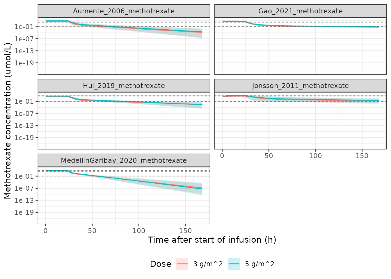
Simulated methotrexate concentration-time profiles by model and dose level. Replicates the layout of Figure 1 of Wang 2023; the horizontal lines are the therapeutic thresholds quoted in that paper’s Introduction.
Steady-state concentration at end of infusion
Wang 2023 Introduction defines Cp,ss as the concentration at the end of the 24 h infusion and quotes the efficacy thresholds: above 65 umol/L for intermediate/high-risk children (the 5.0 g/m^2 arm), above 33 umol/L for low-risk children (the 3.0 g/m^2 arm), and subtherapeutic below 16 umol/L.
The point of the paper is that these six models disagree with one another, so this table is presented as a cross-model comparison rather than as a gate on any single published number.
cpss <- sim |>
  filter(abs(time - 24) < 1e-6) |>
  group_by(model, treatment) |>
  summarise(
    `Median Cp,ss` = median(Cc),
    `P10`          = quantile(Cc, 0.10),
    `P90`          = quantile(Cc, 0.90),
    .groups = "drop"
  )

cpss |>
  knitr::kable(digits = 1,
caption = "Simulated Cp,ss (umol/L) at the end of the 24 h infusion.")| model | treatment | Median Cp,ss | P10 | P90 |
|---|---|---|---|---|
| Aumente_2006_methotrexate | 3 g/m^2 | 52.9 | 30.4 | 80.8 |
| Aumente_2006_methotrexate | 5 g/m^2 | 76.1 | 48.0 | 150.6 |
| Gao_2021_methotrexate | 3 g/m^2 | 26.7 | 21.1 | 35.2 |
| Gao_2021_methotrexate | 5 g/m^2 | 49.4 | 34.6 | 62.0 |
| Hui_2019_methotrexate | 3 g/m^2 | 23.1 | 16.6 | 31.7 |
| Hui_2019_methotrexate | 5 g/m^2 | 43.7 | 30.5 | 51.9 |
| Jonsson_2011_methotrexate | 3 g/m^2 | 53.2 | 15.6 | 107.0 |
| Jonsson_2011_methotrexate | 5 g/m^2 | 95.9 | 30.1 | 191.4 |
| MedellinGaribay_2020_methotrexate | 3 g/m^2 | 35.1 | 30.4 | 40.7 |
| MedellinGaribay_2020_methotrexate | 5 g/m^2 | 56.4 | 51.3 | 67.5 |
# Structural gate: across every model and both dose levels the median Cp,ss
# must land inside the clinically plausible decade for HD-MTX that Wang 2023
# spans in its Introduction (subtherapeutic < 16 umol/L; > 100 umol/L at 24 h
# is supratherapeutic). A mis-transcribed clearance, volume, dose or unit
# conversion moves a whole median out of this band immediately. Deliberately
# asserted on the MEDIAN, never on the cohort extremes, which are not
# reproducible across rxode2 builds.
stopifnot(all(cpss$`Median Cp,ss` > 5), all(cpss$`Median Cp,ss` < 150))

# The 5 g/m^2 arm must exceed the 3 g/m^2 arm for every model (the models are
# linear, so this is exact up to the drawn cohort).
wide <- tidyr::pivot_wider(cpss, id_cols = model, names_from = treatment,
                           values_from = `Median Cp,ss`)
stopifnot(all(wide[["5 g/m^2"]] > wide[["3 g/m^2"]]))
Structural verification
Typical parameter values against the paper’s own text
Wang 2023 Results 3.1 quotes typical values it computed from the same Table 2 equations packaged here. Solving each model at its own development-cohort median (Wang 2023 Table 1) with between-subject variability zeroed must reproduce those numbers. These are exact, deterministic identities – no random draw is involved – so they are asserted tightly.
typical_solve <- function(model_name, covs) {
  ui <- rxode2::zeroRe(rxode2::rxode(readModelDb(model_name)))
  ev <- data.frame(id = 1L, time = c(0, 1), amt = c(1000, NA),
                   dur = c(0.5, NA), evid = c(1L, 0L), cmt = "central")
  ev <- cbind(ev, as.data.frame(covs))
  s <- rxode2::rxSolve(ui, events = ev, returnType = "data.frame",
                       addDosing = FALSE)
  s[1, ]
}

typ <- list(
  Aumente_2006_methotrexate         = list(WT = 24.2, AGE = 5.0),
  Gao_2021_methotrexate             = list(WT = 19.0, CREAT = 26.0),
  Hui_2019_methotrexate             = list(BSA = 0.735, CRCL = 149.9,
                                           AGE = 5.29, OCC = 1L),
  MedellinGaribay_2020_methotrexate = list(BSA = 0.79, WT = 21.2),
  Jonsson_2011_methotrexate         = list(WT = 19.0)
)

typ_res <- do.call(rbind, lapply(names(typ), function(nm) {
  s <- typical_solve(nm, typ[[nm]])
  data.frame(model = nm, cl = s$cl, vc = s$vc)
}))
#> ℹ parameter labels from comments will be replaced by 'label()'
#> ℹ omega/sigma items treated as zero: 'etalcl', 'etalvc', 'etalk12', 'etalk21'
#> ℹ parameter labels from comments will be replaced by 'label()'
#> ℹ omega/sigma items treated as zero: 'etalcl', 'etalq'
#> ℹ parameter labels from comments will be replaced by 'label()'
#> Warning: some etas defaulted to non-mu referenced, possible parsing error: etaiov_cl_1, etaiov_cl_2, etaiov_cl_3, etaiov_cl_4
#> as a work-around try putting the mu-referenced expression on a simple line
#> Warning: some etas defaulted to non-mu referenced, possible parsing error: etaiov_cl_1, etaiov_cl_2, etaiov_cl_3, etaiov_cl_4
#> as a work-around try putting the mu-referenced expression on a simple line
#> ℹ omega/sigma items treated as zero: 'etalcl', 'etalvp', 'etaiov_cl_1', 'etaiov_cl_2', 'etaiov_cl_3', 'etaiov_cl_4'
#> ℹ parameter labels from comments will be replaced by 'label()'
#> ℹ omega/sigma items treated as zero: 'etalcl', 'etalvc', 'etalvp'
#> ℹ parameter labels from comments will be replaced by 'label()'
#> ℹ omega/sigma items treated as zero: 'etalcl', 'etalvc', 'etalq', 'etalvp'

knitr::kable(typ_res, digits = 3,
caption = "Typical CL and Vc at each model's own cohort median.")| model | cl | vc |
|---|---|---|
| Aumente_2006_methotrexate | 4.678 | 11.253 |
| Gao_2021_methotrexate | 6.900 | 20.700 |
| Hui_2019_methotrexate | 7.716 | 19.000 |
| MedellinGaribay_2020_methotrexate | 5.616 | 7.632 |
| Jonsson_2011_methotrexate | 3.515 | 24.130 |
getv <- function(m, col) typ_res[[col]][typ_res$model == m]

stopifnot(
  # "Typical estimates for MTX clearance in the included studies ranged from
  #  3.52 [Jonsson] to 7.73 [Hui] L/h" -- Wang 2023 Results 3.1.
  abs(getv("Jonsson_2011_methotrexate", "cl") - 3.52) < 0.01,
  abs(getv("Hui_2019_methotrexate", "cl") - 7.73) < 0.02,
  # "the typical central volume of distribution ... ranging from 7.5
  #  [Medellin-Garibay] to 24.1 [Jonsson] L" -- same paragraph.
  abs(getv("Jonsson_2011_methotrexate", "vc") - 24.1) < 0.05,
  abs(getv("MedellinGaribay_2020_methotrexate", "vc") - 7.6) < 0.1,
  # Gao 2021 Table 2 typical CL for a 19 kg child at the 26 umol/L reference.
  abs(getv("Gao_2021_methotrexate", "cl") - 6.9) < 0.01
)
Terminal half-life against the analytic eigenvalue
The terminal half-life PKNCA estimates from the simulated curve must agree with the one implied by the model’s own micro-constants. Both sides use the same parameter values, so the only difference is numerical – a tight bound is correct here, and would catch a compartment wired to the wrong state.
analytic_thalf <- function(model_name, covs) {
  s <- typical_solve(model_name, covs)
  k10 <- s$cl / s$vc
  k12 <- s$q / s$vc
  k21 <- s$q / s$vp
  if (!is.null(s$q2) && !is.na(s$q2)) {
    k13 <- s$q2 / s$vc
    k31 <- s$q2 / s$vp2
    A <- matrix(c(-(k10 + k12 + k13), k21, k31,
                  k12, -k21, 0,
                  k13, 0, -k31), nrow = 3, byrow = TRUE)
  } else {
    A <- matrix(c(-(k10 + k12), k21,
                  k12, -k21), nrow = 2, byrow = TRUE)
  }
  lambda <- Re(eigen(A)$values)
  log(2) / abs(max(lambda)) # least-negative eigenvalue = terminal slope
}

thalf_analytic <- vapply(names(typ),
                         function(nm) analytic_thalf(nm, typ[[nm]]),
                         numeric(1))
#> ℹ parameter labels from comments will be replaced by 'label()'
#> ℹ omega/sigma items treated as zero: 'etalcl', 'etalvc', 'etalk12', 'etalk21'
#> ℹ parameter labels from comments will be replaced by 'label()'
#> ℹ omega/sigma items treated as zero: 'etalcl', 'etalq'
#> ℹ parameter labels from comments will be replaced by 'label()'
#> Warning: some etas defaulted to non-mu referenced, possible parsing error: etaiov_cl_1, etaiov_cl_2, etaiov_cl_3, etaiov_cl_4
#> as a work-around try putting the mu-referenced expression on a simple line
#> Warning: some etas defaulted to non-mu referenced, possible parsing error: etaiov_cl_1, etaiov_cl_2, etaiov_cl_3, etaiov_cl_4
#> as a work-around try putting the mu-referenced expression on a simple line
#> ℹ omega/sigma items treated as zero: 'etalcl', 'etalvp', 'etaiov_cl_1', 'etaiov_cl_2', 'etaiov_cl_3', 'etaiov_cl_4'
#> ℹ parameter labels from comments will be replaced by 'label()'
#> ℹ omega/sigma items treated as zero: 'etalcl', 'etalvc', 'etalvp'
#> ℹ parameter labels from comments will be replaced by 'label()'
#> ℹ omega/sigma items treated as zero: 'etalcl', 'etalvc', 'etalq', 'etalvp'
round(thalf_analytic, 2)
#>         Aumente_2006_methotrexate             Gao_2021_methotrexate
#>                             10.00                            115.65
#>             Hui_2019_methotrexate MedellinGaribay_2020_methotrexate
#>                             16.90                              5.88
#>         Jonsson_2011_methotrexate
#>                             45.85
PKNCA validation
Wang 2023 reports no non-compartmental analysis of its own – it reports prediction-error metrics instead – so there is no published NCA table to compare against. The NCA is therefore run as an internal-identity check: PKNCA’s terminal half-life on a typical-value (variability-zeroed) solve must match the analytic eigenvalue computed above.
Running the NCA on the typical-value solve rather than the
full-variability cohort is deliberate: over a cohort with
between-subject variability, the half-life estimate is both
NA-poisoned and tmax-selected, which makes it a poor
gate.
typical_profile <- function(model_name, covs, dose_g_m2 = 3.0) {
  ui <- rxode2::zeroRe(rxode2::rxode(readModelDb(model_name)))
  bsa <- if (!is.null(covs$BSA)) covs$BSA else sqrt(113 * covs$WT / 3600)
  dose_umol <- dose_g_m2 * bsa * 1e6 / MW_MTX

  dosing <- data.frame(
    id = 1L, time = c(0, 0.5),
    amt = c(dose_umol * 0.10, dose_umol * 0.90),
    dur = c(0.5, 23.5), evid = 1L, cmt = "central"
  )
  obs <- data.frame(
    id = 1L,
    time = sort(unique(c(seq(0, 48, by = 0.25), seq(49, 336, by = 1)))),
    amt = NA_real_, dur = NA_real_, evid = 0L, cmt = "central"
  )
  ev <- bind_rows(dosing, obs)
  for (nm in names(covs)) ev[[nm]] <- covs[[nm]]
  ev <- arrange(ev, time, desc(evid))

  s <- rxode2::rxSolve(ui, events = ev, returnType = "data.frame",
                       addDosing = FALSE) |>
    mutate(model = model_name, dose_umol = dose_umol)
  s
}

typ_prof <- bind_rows(lapply(names(typ),
                             function(nm) typical_profile(nm, typ[[nm]])))
#> ℹ parameter labels from comments will be replaced by 'label()'
#> ℹ omega/sigma items treated as zero: 'etalcl', 'etalvc', 'etalk12', 'etalk21'
#> ℹ parameter labels from comments will be replaced by 'label()'
#> ℹ omega/sigma items treated as zero: 'etalcl', 'etalq'
#> ℹ parameter labels from comments will be replaced by 'label()'
#> Warning: some etas defaulted to non-mu referenced, possible parsing error: etaiov_cl_1, etaiov_cl_2, etaiov_cl_3, etaiov_cl_4
#> as a work-around try putting the mu-referenced expression on a simple line
#> Warning: some etas defaulted to non-mu referenced, possible parsing error: etaiov_cl_1, etaiov_cl_2, etaiov_cl_3, etaiov_cl_4
#> as a work-around try putting the mu-referenced expression on a simple line
#> ℹ omega/sigma items treated as zero: 'etalcl', 'etalvp', 'etaiov_cl_1', 'etaiov_cl_2', 'etaiov_cl_3', 'etaiov_cl_4'
#> ℹ parameter labels from comments will be replaced by 'label()'
#> ℹ omega/sigma items treated as zero: 'etalcl', 'etalvc', 'etalvp'
#> ℹ parameter labels from comments will be replaced by 'label()'
#> ℹ omega/sigma items treated as zero: 'etalcl', 'etalvc', 'etalq', 'etalvp'

# PKNCA input: filter ONLY on missing concentrations so the time-zero row
# survives (dropping it triggers the "AUC range starting before the first
# measurement" warning).
nca_conc <- typ_prof |>
  filter(!is.na(Cc)) |>
  mutate(id = model) |>
  select(id, time, Cc, model)

nca_dose <- typ_prof |>
  group_by(model) |>
  summarise(id = first(model), time = 0, amt = first(dose_umol),
            .groups = "drop") |>
  select(id, time, amt, model)

conc_obj <- PKNCA::PKNCAconc(nca_conc, Cc ~ time | model + id,
                             concu = "umol/L", timeu = "h")
dose_obj <- PKNCA::PKNCAdose(nca_dose, amt ~ time | model + id,
                             doseu = "umol")

intervals <- data.frame(
  start = 0, end = Inf,
  cmax = TRUE, tmax = TRUE, auclast = TRUE,
  aucinf.obs = TRUE, half.life = TRUE, clast.obs = TRUE
)

nca_res <- PKNCA::pk.nca(
  PKNCA::PKNCAdata(conc_obj, dose_obj, intervals = intervals)
)
nca_wide <- as.data.frame(nca_res) |>
  filter(PPTESTCD %in% c("cmax", "tmax", "half.life", "auclast", "aucinf.obs")) |>
  select(model, PPTESTCD, PPORRES) |>
  tidyr::pivot_wider(names_from = PPTESTCD, values_from = PPORRES) |>
  mutate(`Analytic t1/2 (h)` = thalf_analytic[model]) |>
  # Rename BY NAME, never positionally via col.names.
  dplyr::rename(
    "Model"              = model,
    "Cmax (umol/L)"      = cmax,
    "Tmax (h)"           = tmax,
    "t1/2 (h), PKNCA"    = half.life,
    "AUClast (umol*h/L)" = auclast,
    "AUCinf (umol*h/L)"  = aucinf.obs
  )

knitr::kable(nca_wide, digits = 2,
             caption = paste("PKNCA parameters on the typical-value solve at",
                             "3 g/m^2, with the analytic terminal half-life",
"for comparison."))| Model | AUClast (umol*h/L) | Cmax (umol/L) | Tmax (h) | t1/2 (h), PKNCA | AUCinf (umol*h/L) | Analytic t1/2 (h) |
|---|---|---|---|---|---|---|
| Aumente_2006_methotrexate | 1229.71 | 46.71 | 24.0 | 9.96 | 1229.71 | 10.00 |
| Gao_2021_methotrexate | 734.90 | 27.19 | 24.0 | 114.77 | 738.78 | 115.65 |
| Hui_2019_methotrexate | 628.83 | 23.73 | 24.0 | 16.84 | 628.83 | 16.90 |
| Jonsson_2011_methotrexate | 1449.26 | 51.02 | 24.0 | 45.68 | 1450.35 | 45.85 |
| MedellinGaribay_2020_methotrexate | 928.46 | 56.47 | 0.5 | 5.91 | 928.46 | 5.88 |
rel_diff <- abs(nca_wide[["t1/2 (h), PKNCA"]] - nca_wide[["Analytic t1/2 (h)"]]) /
  nca_wide[["Analytic t1/2 (h)"]]
names(rel_diff) <- nca_wide$Model
round(100 * rel_diff, 3)
#>         Aumente_2006_methotrexate             Gao_2021_methotrexate
#>                             0.380                             0.764
#>             Hui_2019_methotrexate         Jonsson_2011_methotrexate
#>                             0.376                             0.374
#> MedellinGaribay_2020_methotrexate
#>                             0.477

# Same parameters on both sides -- the difference is pure numerical error in
# the log-linear terminal regression, so this is tight by construction.
stopifnot(all(rel_diff < 0.02))

# Tmax must sit at the end of ONE of the two infusion segments -- 0.5 h (end of
# the 10% loading infusion) or 24 h (end of the 90% maintenance infusion) --
# and never in between. Concentration rises throughout the loading infusion,
# then approaches the much lower maintenance input rate monotonically, so the
# maximum over the whole regimen is attained at one of the two endpoints.
# Which endpoint wins depends on the central volume; see the note below.
stopifnot(all(nca_wide[["Tmax (h)"]] %in% c(0.5, 24)))

# Equivalently and more strongly: Cmax equals the larger of the two
# end-of-segment concentrations, exactly.
endpoint_conc <- typ_prof |>
  filter(time %in% c(0.5, 24)) |>
  group_by(model) |>
  summarise(peak = max(Cc), .groups = "drop")
stopifnot(all(abs(
  endpoint_conc$peak[match(nca_wide$Model, endpoint_conc$model)] -
    nca_wide[["Cmax (umol/L)"]]
) < 1e-6))

# AUCinf must be at least AUClast, and the extrapolated tail must be
# negligible given sampling out to 336 h. Note the comparison is >=, not >:
# for Aumente, Hui and Medellin-Garibay the profile has decayed so far by
# 336 h (Clast of 8e-10, 2e-6 and 3e-16 umol/L respectively) that the
# extrapolated tail vanishes into floating-point precision and AUCinf equals
# AUClast exactly. That is the window doing its job, not a defect.
extrap_frac <- (nca_wide[["AUCinf (umol*h/L)"]] - nca_wide[["AUClast (umol*h/L)"]]) /
  nca_wide[["AUCinf (umol*h/L)"]]
names(extrap_frac) <- nca_wide$Model
round(100 * extrap_frac, 3)
#>         Aumente_2006_methotrexate             Gao_2021_methotrexate
#>                             0.000                             0.526
#>             Hui_2019_methotrexate         Jonsson_2011_methotrexate
#>                             0.000                             0.076
#> MedellinGaribay_2020_methotrexate
#>                             0.000

stopifnot(
  all(nca_wide[["AUCinf (umol*h/L)"]] >= nca_wide[["AUClast (umol*h/L)"]]),
  all(extrap_frac >= 0),
  # Deterministic typical-value solves, so this is tight by construction.
  all(extrap_frac < 0.02)
)
Note the spread of terminal half-lives across the set – roughly 6 h (Medellin-Garibay) to 115 h (Gao). Gao’s is by far the longest because it is the only three-compartment model of the group, and its first peripheral compartment (41 L, reached through an intercompartmental clearance of only 0.255 L/h) drains very slowly. That deep compartment carries little drug, which is why the extrapolated AUC fraction stays under 1% despite the long terminal slope.
Cmax is not always Cp,ss under this regimen
Wang’s regimen infuses 10% of the dose over 0.5 h and the remaining 90% over 23.5 h, so the loading segment runs at roughly five times the maintenance infusion rate. For models with a small central volume the loading segment therefore produces a transient peak that exceeds the end-of-infusion concentration, and Cmax is attained at 0.5 h rather than at 24 h.
In this set that happens for Medellin-Garibay 2020, whose central volume (7.6 L at the cohort median) is the smallest of the six models Wang evaluated: its Cmax is about 56 umol/L at 0.5 h against a Cp,ss of about 35 umol/L at 24 h. Aumente 2006, with the next-smallest volume, is nearly tied between the two endpoints. The remaining models peak at 24 h.
This matters when reading the paper’s therapeutic thresholds: Wang defines Cp,ss as the 24 h value specifically, so for these models Cp,ss is not the maximum concentration the patient experiences.
Published external-evaluation performance
For reference, Wang 2023 Table 3 reports how each model performed against the independent 51-patient cohort. These are the paper’s own results, reproduced here as published; they are not recomputed by this vignette, because the evaluation dataset is not public.
| Model | IPRED median PE (%) | IPRED MPE (%) | IPRED RMSE (%) | PRED median PE (%) | PRED MPE (%) | PRED RMSE (%) |
|---|---|---|---|---|---|---|
| Aumente 2006 | 6.52 | 12.06 | 76.09 | -31.70 | -25.51 | 81.15 |
| Gao 2021 | -25.20 | 1.33 | 63.96 | -26.76 | 3.22 | 72.39 |
| Hui 2019 | -10.43 | 8.78 | 82.96 | -33.23 | -8.24 | 62.88 |
| Medellin-Garibay 2020 | -0.75 | 22.71 | 75.55 | -7.56 | 6.39 | 68.33 |
| Zhang 2010 (not packaged) | 1.16 | 16.00 | 63.39 | -29.92 | 15.62 | 145.92 |
| Jonsson 2011 | 5.25 | 64.44 | 152.25 | 442.04 | 780.87 | 1182.24 |
Wang’s conclusion is that all six models are usable for individual (a posteriori) prediction but too imprecise for a priori model-informed precision dosing without refinement, and that Jonsson 2011 – the only weight-only model, built on a 5-8 g/m^2 cohort that does not overlap the 1-5 g/m^2 evaluation data – fails badly on population predictions.
Assumptions and deviations
Provenance: these are transcriptions from a review
Four of the five models are transcribed from Wang 2023 Table
2, not from their own primary publications, because those
primaries are not open access. Each model file records this in its
reference metadata and each is planned for re-extraction
from its primary. The exception is Gao 2021, which is open access and is
encoded from the primary.
Wang 2023 Table 2 mis-transcribes the Gao 2021 row (twice)
Gao 2021 being open access made a direct comparison possible, and it found two errors in Wang’s rendering:
- Wang prints the CL between-subject CV as 17.9%; Gao’s own Table 2 says 17.5%.
- Wang places the second eta on V2 in its equation
column and calls it V1 in its IIV column – disagreeing
with itself. Gao places it on Q1, and says so twice
(Table 2 populates the
CV for IIVcell on the Q1 row, and the Results state that adding serum creatinine “reduced the variability of Q1 by 29.2%”).
Gao_2021_methotrexate.R follows the Gao primary. This
finding is the direct evidence that Wang’s Table 2 is not a reliable
transcription source, and is why the other four models carry
re-extraction notes.
Wang’s Table 1 has a similar slip in the Gao column. It prints AST as
26.0 (8.0-135.0) U/L, which is Gao’s serum-creatinine row in umol/L.
Gao’s own Table 1 gives AST 22.6 (7.0-319.0) U/L. The
population metadata of Gao_2021_methotrexate.R
is therefore taken from Gao’s Table 1, not Wang’s.
Gao 2021: the serum-creatinine term is unbounded
Gao’s creatinine effect is linear, not a power term:
CL = CL_typical * (1 + (Scr - 26) * (-0.0097)). It reaches
zero at Scr = 129.1 umol/L and goes negative above that
– inside Gao’s own reported creatinine range (Gao Table 1: 8.0-135.0
umol/L). The published equation is reproduced as printed rather than
clamped. Simulations must keep CREAT below about 129
umol/L; the cohort here has a maximum well below it.
Gao’s own Table 2 footnote writes the equation as
[CL = CL_typical x ((SCr-26) x 0.0097)], which is garbled –
it drops both the 1 + and the minus sign, and would make
clearance zero at the reference value. Wang’s rendering is the coherent
one and is used.
Hui 2019: an unresolvable parenthesisation
Wang 2023 Table 2 prints Hui’s renal term as
(eGFR x 1.73/192 x BSA)^0.256. Read with ordinary
left-to-right precedence – and a 400 dpi render confirms an inline
solidus rather than a fraction bar – this is
(eGFR * 1.73 * BSA / 192)^0.256, which is what is encoded.
That reading also behaves like a properly normalised covariate: at the
evaluation cohort’s median eGFR (149.9) and Hui’s median BSA (0.735) the
bracket evaluates to 0.993, i.e. centred at approximately 1.
The alternative grouping (eGFR x 1.73)/(192 x BSA)
cannot be excluded without the primary and would raise typical clearance
by about 17%. Hui 2019 is planned for re-extraction.
Jonsson 2011: the residual error is assumed, not published
Wang 2023 Table 2 records Jonsson’s residual variability as
NR (not reported), and Wang supplied one for the
evaluation (Methods 2.3: “a proportional error of 30% was assumed for
the residual variability if the models did not report this
information”). The packaged model carries
propSd <- fixed(0.30) so it reproduces the model Wang
actually evaluated, but this is not a Jonsson 2011
estimate and must not be read as one. It is wrapped in
fixed() precisely because nothing in either source
estimated it.
Aumente 2006: the 10-year boundary is undefined
Wang 2023 Table 2 gives one pair of CL/V1 equations for “age > 10 years” and another for “age < 10 years”, leaving age exactly 10.0 undefined (both inequalities are strict). This implementation assigns age exactly 10 to the older stratum. The choice changes the prediction only for a subject recorded at exactly 10.0 years.
Hui 2019: the occasion count is an implementation choice
Wang reports a single shared between-occasion variance (14.9% CV) for
clearance but does not state how many occasions the primary modelled.
Four occasion slots are provided, all carrying that same published
variance with only the first estimable (the NONMEM
OMEGA BLOCK(1) SAME idiom). The slot count invents no
parameter value; it only bounds how many distinct courses a user can
encode. Set OCC = 1 for a single-course simulation.
Wang’s Results also mis-reads this row once, describing the 14.9% as
an inter-individual effect; Table 2’s own column header
(IIV (%) (IOV (%))) makes 14.9% the inter-occasion value
and 14.3% the inter-individual one, and Table 2 is followed here.
Zhang 2010 is deferred, not dropped
The sixth model Wang evaluated, Zhang 2010 (Int J Clin Pharmacol Ther 48:11-21, doi:10.5414/cpp48011), is not packaged in this release. Its clearance equation as printed by Wang is
CL (L/h) = (5.04 * (1 - 0.278 * Gender) * BSA^0.777 + (OH/100)^0.514) * exp(eta_CL)and two things in it cannot be resolved from any available source:
-
OH– “pre-chemotherapy alkalinization volume” – has no stated units. The term is additive to the BSA term, in L/h, so the scale matters enormously: at a typical pre-hydration volume of ~1500 mL the term contributes about 4 L/h, comparable to the entire BSA term and roughly doubling typical clearance. Zhang’s own abstract presents 5.04 L/h as the typical clearance, which is only consistent with theOHterm being near zero. The two readings differ about two-fold and cannot be told apart from the available sources. -
Gender’s reference category is unstated.(1 - 0.278 * Gender)meansGender = 1lowers clearance by 27.8%, but neither Wang nor Zhang’s abstract says which sex that is. A flip changes typical clearance by ~38%.
The Zhang 2010 primary is not open access. Rather than ship a model with an assumed covariate scale that can swing clearance two-fold, the Zhang 2010 model is deferred and will be extracted from its primary, where both the units and the coding will be stated. Its row is retained in the published performance table above for completeness.