Tapentadol (Watson 2019)

Model and source

• Citation: Watson E, Khandelwal A, Freijer J, van den Anker J, Lefeber C, Eerdekens M. Population pharmacokinetic modeling to facilitate dose selection of tapentadol in the pediatric population. J Pain Res. 2019;12:2835-2850. doi:10.2147/JPR.S208454

• Description: One-compartment population PK model for tapentadol oral solution in 92 children and adolescents aged 2 to <18 years with moderate-to-severe acute postsurgical pain (Watson 2019). First-order absorption from a depot compartment into the central compartment preceded by an absorption lag time, and first-order elimination; clearance and volume are apparent (CL/F, V/F) because only the oral solution was studied. Body weight is the only retained covariate, entering CL/F and V/F as a power function normalized to the 45 kg population median with exponents estimated (0.638 and 0.847) rather than fixed to the allometric 0.75 and 1. Inter-individual variability is exponential on CL/F, V/F and Ka with a full 3x3 correlation block, and the residual error is combined proportional plus additive. Age, sex, creatinine clearance, AST, ALT, ALP and bilirubin were screened by stepwise covariate modeling and none survived backward elimination, so the final model equals the weight-only base model.

• Article: https://doi.org/10.2147/JPR.S208454 (open access; J Pain Res. 2019;12:2835-2850, PMC6800464)

Watson 2019 is the first population PK analysis of tapentadol in children. Two open-label single-dose phase 2 trials (NCT01729728, NCT01134536) gave a 1.0 mg/kg tapentadol oral solution (OS) dose to patients aged 2 to <18 years with acute postsurgical pain. The final model is a one-compartment model with first-order absorption from a depot compartment, an absorption lag time, and first-order elimination, with body weight as the only retained covariate on CL/F and V/F. The fitted model was then used to pick a dose (1.25 mg/kg q4h) for a confirmatory efficacy trial by matching pediatric steady-state exposure to the adult exposure at 50-100 mg immediate release (IR) q4h.

Population

Population metadata recorded with the model (Watson 2019 Table 1 and Methods).

Field	Value
species	human
n_subjects	92
n_studies	2
n_observations	424 tapentadol serum concentrations used for model building and evaluation, from 462 samples drawn in 109 treated patients (Watson 2019 Methods, ‘Data set’)
age_range	2 to <18 years; group medians (range) 15 (12-17), 9 (6-11) and 3 (2-5) years; cohort mean (SD) 11 (4.7) years
age_median	11 years (mean); stratified as 12 to <18 years (n=44), 6 to <12 years (n=33) and 2 to <6 years (n=15)
weight_range	12.7-80 kg; group medians (range) 60 (41-80), 29.5 (20.2-58) and 16.3 (12.7-19.5) kg; cohort mean (SD) 43 (19.7) kg
weight_median	45 kg (the covariate reference weight used for CL/F and V/F in Table 2)
sex_female_pct	53.3
disease_state	Moderate-to-severe acute postsurgical pain
dose_range	Single tapentadol oral solution dose of 1.0 mg/kg body weight; the 4 mg/mL strength for patients <20 kg and the 20 mg/mL strength for patients >=20 kg, with total dose capped at 75 mg
regions	Canada, Spain and the USA (NCT01134536); single-country sites for NCT01729728 (Quorum Review IRB, Seattle, USA)
notes	Pooled from two open-label single-dose phase 2 PK trials, NCT01729728 (n=56) and NCT01134536 (n=36); baseline demographics by trial and age stratum are in Table 1. Patients were recruited in a staggered fashion by descending age group. Of 109 treated patients, 17 (38 samples, 8%) were excluded for vomiting within 3 hrs of intake or for an incomplete dose. About 3% of samples were below the 0.2 ng/mL LOQ and were excluded rather than imputed or replaced. Body weight and age were highly correlated (r=0.92), which is why weight alone suffices as the size descriptor. Sampling intensity differed by age group: 8 timed samples for 12 to <18 years, 4 windowed samples for 6 to <12 years, 2 windowed samples for 3-5 years and 4 timed samples for 2-year-olds. The tapentadol-O-glucuronide metabolite was assayed but is not modelled here; the paper models only the active moiety because the glucuronide is not analgesically active. Estimation used NONMEM 7.2 FOCE with interaction.

424 tapentadol serum concentrations from 92 patients entered the analysis, drawn from 462 samples in 109 treated patients; 17 patients (38 samples, 8%) were excluded for vomiting within 3 hrs of dosing or for an incomplete dose, and about 3% of samples fell below the 0.2 ng/mL LOQ and were excluded rather than imputed. Patients were stratified into three age groups whose Table 1 combined median (range) weights were 60 (41-80) kg for 12 to <18 years (n=44), 29.5 (20.2-58) kg for 6 to <12 years (n=33), and 16.3 (12.7-19.5) kg for 2 to <6 years (n=15). Weight and age were highly correlated (r=0.92), which is why weight alone serves as the size descriptor. The cohort was 53.3% female. The same metadata is available programmatically via readModelDb("Watson_2019_tapentadol")()$population.

Source trace

Each ini() entry in inst/modeldb/specificDrugs/Watson_2019_tapentadol.R carries an in-file comment naming its source. They are collected here.

Equation / parameter	Value	Source location
lka (Ka)	2.03 1/h	Table 2, row Ka (h-1) (RSE 16.5%)
ltlag (TLAG)	0.247 h	Table 2, row TLAG (h) (RSE 0.7%)
lcl (CL/F at 45 kg)	170 L/h	Table 2, row CL/F (L/h) (RSE 3.3%)
lvc (V/F at 45 kg)	685 L	Table 2, row V/F (L) (RSE 4.5%)
e_wt_cl	0.638	Table 2, row Exponent CL-WT (RSE 11.1%)
e_wt_vc	0.847	Table 2, row Exponent V-WT (RSE 10.2%)
etalcl variance	0.048	Table 2, row IIV CL/F (omega^2) (RSE 32.1%)
etalvc variance	0.024	Table 2, row IIV V/F (omega^2) (RSE 61.5%)
etalka variance	1.99	Table 2, row IIV Ka (omega^2) (RSE 32.2%)
cov(etalcl, etalvc)	0.03	Table 2, row Cov CL/F-V/F (RSE 46.1%)
cov(etalcl, etalka)	0.009	Table 2, row Cov CL/F-Ka (RSE 614.5%)
cov(etalvc, etalka)	-0.072	Table 2, row Cov V/F-Ka (RSE 93.6%)
addSd	0.181 ng/mL	Table 2, row Additive error (ng/mL) (RSE 39.1%)
propSd	0.329	Table 2, row Proportional error (sigma) (RSE 8.7%)
Reference weight 45 kg	n/a	Table 2 caption: “Estimates of CL/F and V/F relate to a reference weight of 45 kg”
IIV form Pi = Ptv * exp(eta_i)	n/a	Methods, “Population PK modeling / Model development”
Residual form Co = Cp*(1+eps1) + eps2	n/a	Methods, “Population PK modeling / Model development”
Covariate form PTV = theta*(x/xref)^n	n/a	Methods, “Covariate analysis”
1-cmt, first-order absorption + lag	n/a	Results, “The final population model was best described as a 1-compartment model with linear oral absorption from a dose compartment into the central compartment, with a lag time and linear elimination”
Full 3x3 IIV correlation block	n/a	Results, “Interindividual variability was best described using a full correlation matrix between the parameters”

Internal consistency of Table 2

Table 2 reports the IIV on the variance / covariance scale while the Results prose quotes the same block as percentages and correlations. Both readings are recovered exactly from the packaged block, which also confirms that no log(1 + CV^2) conversion belongs here.

om <- ui$omega
stopifnot(identical(dim(om), c(3L, 3L)))

omega_chk <- tibble::tibble(
  Quantity = c("SD etalcl", "SD etalvc", "SD etalka", "corr CL-V", "corr CL-Ka", "corr V-Ka"),
  Reported = c(21.8, 15.5, 141.1, 0.88, 0.03, -0.33),
  Model = c(sqrt(diag(om)) * 100, stats::cov2cor(om)[lower.tri(om)])
) |>
  mutate(Difference = Model - Reported)

knitr::kable(omega_chk, digits = 3, caption = "Watson 2019 Results prose vs the packaged OMEGA block.")

Watson 2019 Results prose vs the packaged OMEGA block.

Quantity	Reported	Model	Difference
SD etalcl	21.80	21.909	0.109
SD etalvc	15.50	15.492	-0.008
SD etalka	141.10	141.067	-0.033
corr CL-V	0.88	0.884	0.004
corr CL-Ka	0.03	0.029	-0.001
corr V-Ka	-0.33	-0.329	0.001

# The block must be positive definite or rxode2's Cholesky sampler cannot draw
# from it. This is arithmetic on fixed numbers, so an exact bound is correct.
stopifnot(
  all(eigen(om, only.values = TRUE)$values > 0),
  max(abs(omega_chk$Difference[1:3])) < 0.15,
  max(abs(omega_chk$Difference[4:6])) < 0.005
)

Deterministic structural checks

These compare the packaged model against numbers Watson 2019 prints outside Table 2. They involve no simulation and no random draw, so exact tolerances are appropriate.

cl_at <- function(wt) 170 * (wt / 45)^0.638
v_at <- function(wt) 685 * (wt / 45)^0.847

# Discussion, "Population PK model": "the mean population clearance for a 71-kg
# subject is 227 L/h".
cl71 <- cl_at(71)

# Results: median empirical Bayesian estimates of weight-normalised CL/F and V/F
# per age group, against the typical-value prediction at each group's Table 1
# median weight. Figure 5 plots these against the fitted power function.
ebe <- tibble::tribble(
  ~group, ~wt_median, ~clkg_paper, ~vkg_paper,
  "12 to <18 y", 60.0, 3.45, 14.54,
  "6 to <12 y", 29.5, 4.47, 16.57,
  "2 to <6 y", 16.3, 5.28, 18.03
) |>
  mutate(
    clkg_model = cl_at(wt_median) / wt_median,
    vkg_model = v_at(wt_median) / wt_median,
    cl_pct = 100 * (clkg_model - clkg_paper) / clkg_paper,
    v_pct = 100 * (vkg_model - vkg_paper) / vkg_paper
  )

ebe |>
  select(group, wt_median, clkg_paper, clkg_model, cl_pct, vkg_paper, vkg_model, v_pct) |>
  rename(
    "Age group" = group,
    "Median WT (kg)" = wt_median,
    "CL/F paper (L/h/kg)" = clkg_paper,
    "CL/F model (L/h/kg)" = clkg_model,
    "CL/F % diff" = cl_pct,
    "V/F paper (L/kg)" = vkg_paper,
    "V/F model (L/kg)" = vkg_model,
    "V/F % diff" = v_pct
  ) |>
  knitr::kable(digits = 2, caption = "Watson 2019 Results median empirical-Bayes CL/F and V/F per kg vs the typical-value model prediction at each group's median weight (Figure 5).")

Watson 2019 Results median empirical-Bayes CL/F and V/F per kg vs the typical-value model prediction at each group’s median weight (Figure 5).

Age group	Median WT (kg)	CL/F paper (L/h/kg)	CL/F model (L/h/kg)	CL/F % diff	V/F paper (L/kg)	V/F model (L/kg)	V/F % diff
12 to <18 y	60.0	3.45	3.40	-1.33	14.54	14.57	0.18
6 to <12 y	29.5	4.47	4.40	-1.53	16.57	16.24	-2.00
2 to <6 y	16.3	5.28	5.46	3.34	18.03	17.78	-1.38

cat(sprintf("CL/F at 71 kg: model %.1f L/h vs paper 227 L/h\n", cl71))
#> CL/F at 71 kg: model 227.4 L/h vs paper 227 L/h

stopifnot(
  # Reproduces the Discussion's 71-kg clearance to the printed precision.
  abs(cl71 - 227) < 1,
  # The paper's values are medians of empirical-Bayes estimates, which sit close
  # to but not exactly on the typical-value curve; 3.3% is the worst realised.
  max(abs(ebe$cl_pct)) < 6,
  max(abs(ebe$v_pct)) < 6
)

Reproducing both weight-normalised series at all three group medians constrains both reference values and both estimated exponents simultaneously: a mis-transcribed exponent would tilt the three weights against each other, and a mis-transcribed CL/F or V/F would shift all three together.

Virtual cohort

The observed data are not public. The cohort below approximates the trial demographics in Table 1: three age strata, with weights drawn log-normally about each stratum’s published median and rejected and redrawn (not clipped) until they fall inside the published range. Clipping with pmin/pmax would pile subjects onto the band edges and bias the exposure distribution, so the band is treated as the sampling definition.

# set.seed() seeds R's RNG. It does NOT seed rxode2's simulation RNG, and
# rxode2's streams are partitioned per solver thread -- so this cohort is
# reproducible here and different on a machine with a different thread count.
# Every assertion below is therefore written to hold for any cohort the model
# can produce.
set.seed(20190101)

N_PER_GROUP <- 200L # cap is 200 per arm

# Reject-and-redraw within the published weight band; oversample generously so
# the draw is bounded rather than an open-ended while loop.
sample_wt <- function(n, med, lo, hi, sdlog) {
  draw <- stats::rlnorm(40L * n, log(med), sdlog)
  keep <- draw[draw >= lo & draw <= hi]
  stopifnot(length(keep) >= n)
  keep[seq_len(n)]
}

strata <- tibble::tribble(
  ~group, ~med, ~lo, ~hi, ~sdlog,
  "12 to <18 y", 60.0, 41.0, 80.0, 0.15,
  "6 to <12 y", 29.5, 20.2, 58.0, 0.22,
  "2 to <6 y", 16.3, 12.7, 19.5, 0.11
)

# Observation grid. The Ka IIV is enormous (omega = 141% CV), so ka spans
# roughly 0.07-52 1/h across the cohort: a linear early grid would miss Tmax
# for the fast absorbers and understate AUC. The early grid is therefore
# log-spaced, and the window runs to 72 h so the ~7% of subjects whose ka falls
# below kel (flip-flop absorption) are still followed to completion.
obs_grid <- sort(unique(c(
  0,
  exp(seq(log(0.02), log(2), length.out = 22)),
  seq(2.25, 15, by = 0.25),
  seq(16, 72, by = 1),
  c(0.25, 0.5, 1, 2, 4, 6, 11, 15) # the protocol sampling times for 12 to <18 y
)))

make_cohort <- function(n, group, med, lo, hi, sdlog, dose_mg_kg, id_offset) {
  subj <- tibble::tibble(
    id = id_offset + seq_len(n),
    WT = sample_wt(n, med, lo, hi, sdlog),
    group = group
  ) |>
    # Protocol: 1.0 mg/kg, total dose not to exceed 75 mg (Methods, "Clinical
    # trial design and patient population").
    mutate(dose_mg = pmin(dose_mg_kg * WT, 75))

  dosing <- subj |>
    mutate(time = 0, amt = dose_mg, evid = 1L, cmt = "depot")

  obs <- subj |>
    tidyr::crossing(time = obs_grid) |>
    mutate(amt = NA_real_, evid = 0L, cmt = "central")

  dplyr::bind_rows(dosing, obs) |>
    dplyr::arrange(id, time, dplyr::desc(evid))
}

events <- dplyr::bind_rows(
  make_cohort(N_PER_GROUP, strata$group[1], strata$med[1], strata$lo[1], strata$hi[1], strata$sdlog[1], 1.0, 0L),
  make_cohort(N_PER_GROUP, strata$group[2], strata$med[2], strata$lo[2], strata$hi[2], strata$sdlog[2], 1.0, 200L),
  make_cohort(N_PER_GROUP, strata$group[3], strata$med[3], strata$lo[3], strata$hi[3], strata$sdlog[3], 1.0, 400L)
)

stopifnot(
  !anyDuplicated(unique(events[, c("id", "time", "evid")])),
  dplyr::n_distinct(events$id) == 3L * N_PER_GROUP
)

events |>
  filter(evid == 1L) |>
  group_by(group) |>
  summarise(n = n(), `median WT` = median(WT), `min WT` = min(WT), `max WT` = max(WT),
            `median dose (mg)` = median(dose_mg), .groups = "drop") |>
  knitr::kable(digits = 1, caption = "Simulated cohort weights by age stratum; compare Watson 2019 Table 1 (combined).")

Simulated cohort weights by age stratum; compare Watson 2019 Table 1 (combined).

group	n	median WT	min WT	max WT	median dose (mg)
12 to <18 y	200	59.7	41.5	79.7	59.7
2 to <6 y	200	16.3	12.7	19.4	16.3
6 to <12 y	200	29.4	20.2	52.8	29.4

Simulation

mod <- readModelDb("Watson_2019_tapentadol")
sim <- rxode2::rxSolve(mod, events = events, keep = c("group", "WT", "dose_mg")) |>
  as.data.frame()

stopifnot(nrow(sim) > 0L)

# By 72 h the profile has decayed ~10 orders of magnitude below Cmax, where the
# ODE solver's absolute tolerance leaves round-off of either sign; a handful of
# points come back at around -1e-8 ng/mL. PKNCA's lambda-z regression takes
# log(), so those are floored to zero -- but only after asserting the excursion
# is negligible RELATIVE TO Cmax. A genuinely negative concentration (a real
# solver failure, or a mis-signed rate constant) breaks this bound instead of
# being silently zeroed. Realised ratio was 2.3e-10; the bound leaves four
# orders of magnitude of headroom, so it holds for any cohort while still
# being able to go red.
cc_neg <- sim$Cc[!is.na(sim$Cc) & sim$Cc < 0]
cmax_all <- max(sim$Cc, na.rm = TRUE)
cat(sprintf(
  "negative Cc points: %d of %d; worst |Cc|/Cmax = %.3g\n",
  length(cc_neg), sum(!is.na(sim$Cc)),
  if (length(cc_neg)) abs(min(cc_neg)) / cmax_all else 0
))
#> negative Cc points: 2 of 81000; worst |Cc|/Cmax = 2.21e-10
stopifnot(
  cmax_all > 0,
  length(cc_neg) == 0L || abs(min(cc_neg)) < 1e-6 * cmax_all
)
sim$Cc <- pmax(sim$Cc, 0)

Replicate published figures

# Figure 3 shows the 95% prediction interval, which in the paper includes
# residual error; `sim` is the rxode2 simulated observation (IIV + residual
# error), while `Cc` is the error-free individual prediction.
sim |>
  filter(!is.na(Cc), time <= 15) |>
  group_by(group, time) |>
  summarise(
    Q025 = quantile(sim, 0.025, na.rm = TRUE),
    Q50 = quantile(sim, 0.50, na.rm = TRUE),
    Q975 = quantile(sim, 0.975, na.rm = TRUE),
    .groups = "drop"
  ) |>
  ggplot(aes(time, Q50)) +
  geom_ribbon(aes(ymin = pmax(Q025, 0.05), ymax = Q975), alpha = 0.25, fill = "steelblue") +
  geom_line(colour = "firebrick", linewidth = 0.8) +
  facet_wrap(~group) +
  scale_y_log10() +
  labs(
    x = "Time (h)", y = "Tapentadol serum concentration (ng/mL)",
    title = "Single 1.0 mg/kg oral solution dose",
    caption = "Median and 95% prediction interval. Replicates Figures 1 and 3 of Watson 2019."
  ) +
  theme_bw()
#> Warning in transformation$transform(x): NaNs produced
#> Warning in scale_y_log10(): log-10 transformation introduced infinite values.
#> Warning in transformation$transform(x): NaNs produced
#> Warning in scale_y_log10(): log-10 transformation introduced infinite values.
#> Warning: Removed 2 rows containing missing values or values outside the scale range
#> (`geom_line()`).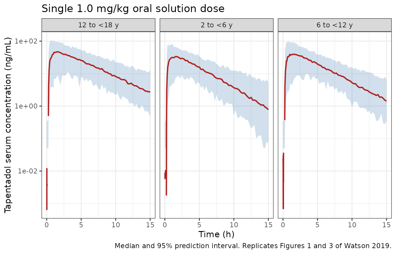

Replicates Figure 1 / Figure 3 of Watson 2019: simulated tapentadol serum concentration versus time after a single 1.0 mg/kg oral-solution dose, by age stratum, over the 15 h trial sampling window.

per_subject <- sim |>
  distinct(id, group, WT) |>
  mutate(cl_ind = cl_at(WT), clkg_ind = cl_ind / WT)

curve_df <- tibble::tibble(WT = seq(12, 82, length.out = 200)) |>
  mutate(cl = cl_at(WT), clkg = cl / WT)

p_left <- ggplot(per_subject, aes(WT, clkg_ind)) +
  geom_point(aes(colour = group), alpha = 0.5, size = 1) +
  geom_line(data = curve_df, aes(WT, clkg), linewidth = 0.9) +
  geom_point(data = ebe, aes(wt_median, clkg_paper), shape = 4, size = 4, stroke = 1.2) +
  labs(x = "Body weight (kg)", y = "CL/F (L/h/kg)", colour = NULL,
       title = "Weight-normalised CL/F") +
  theme_bw() + theme(legend.position = "bottom")

p_right <- ggplot(per_subject, aes(WT, cl_ind)) +
  geom_point(aes(colour = group), alpha = 0.5, size = 1) +
  geom_line(data = curve_df, aes(WT, cl), linewidth = 0.9) +
  labs(x = "Body weight (kg)", y = "CL/F (L/h)", colour = NULL,
       title = "Total CL/F") +
  theme_bw() + theme(legend.position = "bottom")

print(p_left)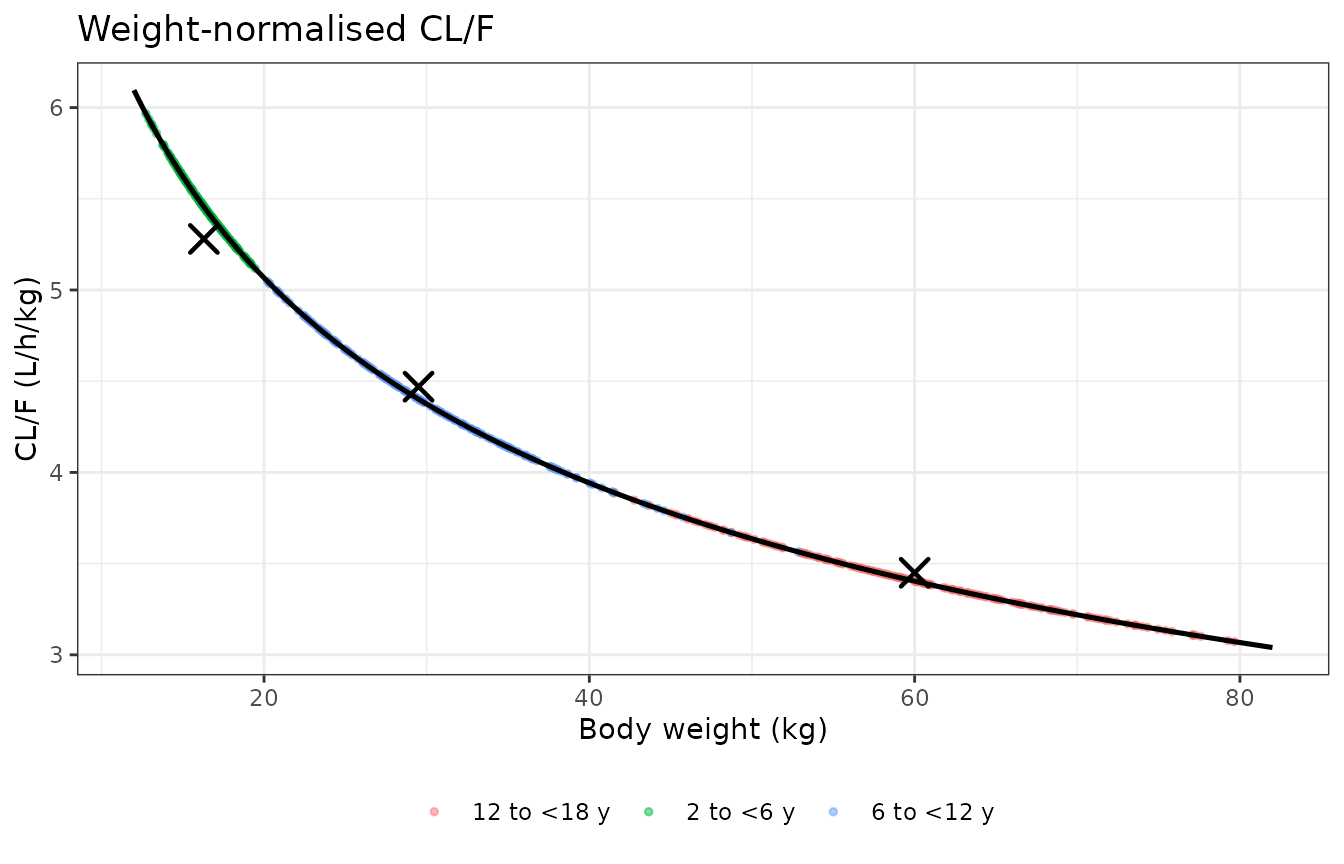

Replicates Figure 5 of Watson 2019: weight-normalised apparent clearance (left) and total apparent clearance (right) versus body weight, with the fitted power function overlaid and the published per-group median empirical-Bayes estimates marked.

print(p_right)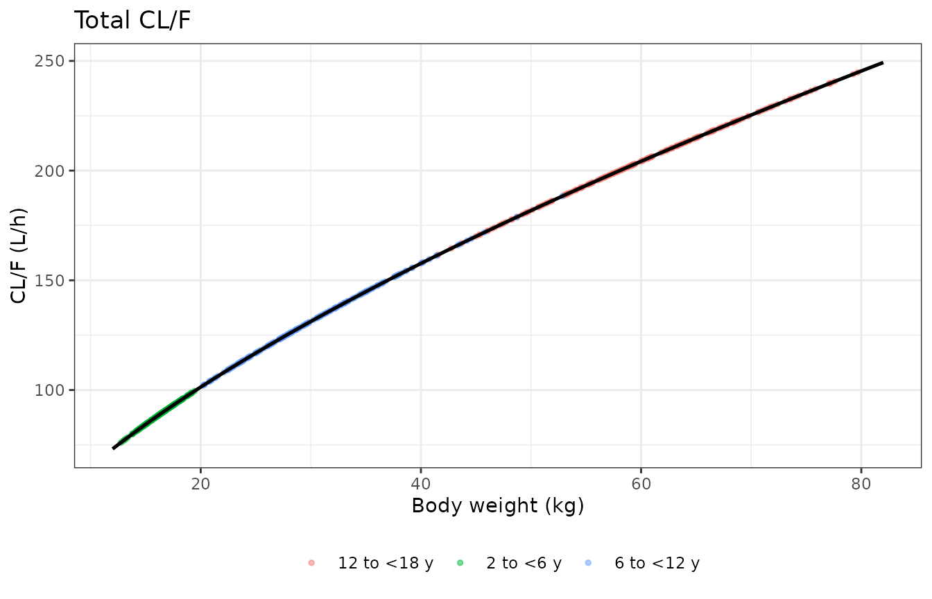

Replicates Figure 5 of Watson 2019: weight-normalised apparent clearance (left) and total apparent clearance (right) versus body weight, with the fitted power function overlaid and the published per-group median empirical-Bayes estimates marked.

The left panel reproduces the paper’s central claim that weight-normalised CL/F decreases with weight (and therefore age) while total CL/F increases, which is what drives the lower exposures in the youngest stratum. The crosses mark the published per-group median empirical-Bayes values from the Results text.

PKNCA validation

Single dose: the mass-balance identity

For a linear model AUC(0-inf) * CL/F = Dose, exactly. This is the packaged model checked against its own closed form, so the residual is pure numerical integration error and a tight bound is the correct assertion.

# Only !is.na(Cc) -- adding `time > 0` or `Cc > 0` would drop the time-zero row
# that PKNCA needs to anchor AUC0-*.
sim_nca <- sim |>
  filter(!is.na(Cc)) |>
  select(id, time, Cc, group)

# Guarantee a time = 0 row per subject; pre-dose Cc = 0 is correct for an
# extravascular dose.
sim_nca <- dplyr::bind_rows(
  sim_nca,
  sim_nca |> distinct(id, group) |> mutate(time = 0, Cc = 0)
) |>
  distinct(id, group, time, .keep_all = TRUE) |>
  arrange(id, group, time)

dose_df <- events |>
  filter(evid == 1L) |>
  select(id, time, amt, group)

conc_obj <- PKNCA::PKNCAconc(sim_nca, Cc ~ time | group + id, concu = "ng/mL", timeu = "h")
dose_obj <- PKNCA::PKNCAdose(dose_df, amt ~ time | group + id, doseu = "mg")

intervals_sd <- data.frame(
  start = 0, end = Inf,
  cmax = TRUE, tmax = TRUE, aucinf.obs = TRUE, auclast = TRUE, half.life = TRUE
)

nca_sd <- PKNCA::pk.nca(PKNCA::PKNCAdata(conc_obj, dose_obj, intervals = intervals_sd))

# The identity uses each subject's INDIVIDUAL CL/F, which rxSolve returns as a
# `cl` column -- not the typical-value CL at that weight. With 21.9% CV of IIV
# on CL/F the two differ per subject, and substituting the typical value turns a
# check that holds to 0.2% into one that spans 0.67-1.52 and tests nothing.
ind_par <- sim |>
  group_by(id) |>
  summarise(WT = first(WT), dose_mg = first(dose_mg), cl = first(cl),
            ka = first(ka), kel = first(kel), .groups = "drop")
stopifnot(nrow(ind_par) == 3L * N_PER_GROUP)

nca_wide <- as.data.frame(nca_sd$result) |>
  filter(PPTESTCD %in% c("cmax", "tmax", "aucinf.obs", "half.life")) |>
  select(id, group, PPTESTCD, PPORRES) |>
  tidyr::pivot_wider(names_from = PPTESTCD, values_from = PPORRES) |>
  left_join(ind_par, by = "id") |>
  # AUC in ng*h/mL, dose in mg, CL in L/h -> Dose/CL is mg/L = 1000 ng/mL
  mutate(auc_identity = aucinf.obs * cl / (dose_mg * 1000))

stopifnot(nrow(nca_wide) == 3L * N_PER_GROUP, !anyNA(nca_wide$aucinf.obs))

cat(sprintf(
  "AUCinf * CL/F / Dose: median %.5f, 5th pct %.5f, 95th pct %.5f, max deviation %.3f%%\n",
  median(nca_wide$auc_identity),
  quantile(nca_wide$auc_identity, 0.05),
  quantile(nca_wide$auc_identity, 0.95),
  100 * max(abs(nca_wide$auc_identity - 1))
))
#> AUCinf * CL/F / Dose: median 0.99894, 5th pct 0.99850, 95th pct 0.99959, max deviation 0.189%
cat(sprintf("subjects with ka < kel (flip-flop absorption): %.1f%%\n",
            100 * mean(nca_wide$ka < nca_wide$kel)))
#> subjects with ka < kel (flip-flop absorption): 6.0%

# Both sides of this identity come from the SAME draw, so the residual is pure
# numerical-integration error, not cohort noise -- a tight bound is correct here
# and should not be loosened. Realised median deviation 0.09% and max 0.17%; the
# bounds leave headroom for a cohort that draws an even slower absorber (whose
# AUCinf extrapolation from a 72 h window carries the most error) while still
# going red on any unit or scaling error, which would move these by tens of
# percent.
stopifnot(
  abs(median(nca_wide$auc_identity) - 1) < 0.005,
  max(abs(nca_wide$auc_identity - 1)) < 0.02
)

Simulated single-dose (1.0 mg/kg) NCA medians by age stratum. Watson 2019 publishes no observed NCA table, so these are reported for orientation rather than comparison.

Age group	Cmax (ng/mL)	Tmax (h)	AUC0-inf (ng*h/mL)	t1/2 (h)
12 to <18 y	52.53	1.29	295.40	2.96
2 to <6 y	39.69	1.29	187.77	2.31
6 to <12 y	46.75	1.29	229.49	2.56

Watson 2019 reports no observed single-dose NCA table, so there is nothing to compare these against; the comparison against published values is the steady-state AUC below. Note that for about 6-7% of subjects ka falls below kel, so their terminal slope reflects absorption rather than elimination and the fitted t1/2 is an absorption half-life. That is a genuine property of a model with 141% CV on Ka, not an artefact.

Steady state: reproducing Table 3

Table 3 gives the simulated median steady-state AUC for each age stratum at 1.0, 1.25 and 1.5 mg/kg q4h. The nine published values are exactly dose-proportional (294.91 x 1.25 = 368.64; x 1.5 = 442.36, and likewise for the other strata), which establishes that the paper applied no dose cap in these simulations even though the trials capped the single dose at 75 mg. The reproduction below therefore does not cap either.

The published values are medians over a virtual cohort whose weight distribution came from CDC growth charts and is not published, so they are compared against a deterministic typical-value solve at each stratum’s Table 1 median weight (rxode2::zeroRe()), which is reproducible across machines.

TAU <- 4
N_DOSE <- 30L # q4h for 5 days
t_last <- TAU * (N_DOSE - 1L) # 116 h

ss_arms <- tidyr::crossing(
  strata |> select(group, wt = med),
  dose_mg_kg = c(1.0, 1.25, 1.5)
) |>
  mutate(
    id = dplyr::row_number(),
    dose_mg = dose_mg_kg * wt,
    treatment = sprintf("%.2f mg/kg, %s", dose_mg_kg, group)
  )

ss_obs_grid <- sort(unique(c(
  seq(0, t_last, by = TAU),
  seq(t_last, t_last + TAU, by = 0.02) # dense over the final interval
)))

ss_dosing <- ss_arms |>
  tidyr::crossing(time = TAU * seq(0L, N_DOSE - 1L)) |>
  mutate(amt = dose_mg, evid = 1L, cmt = "depot")

ss_events <- dplyr::bind_rows(
  ss_dosing,
  ss_arms |>
    tidyr::crossing(time = ss_obs_grid) |>
    mutate(amt = NA_real_, evid = 0L, cmt = "central")
) |>
  rename(WT = wt) |>
  arrange(id, time, desc(evid))

sim_ss <- rxode2::rxSolve(
  rxode2::zeroRe(mod),
  events = ss_events,
  keep = c("treatment", "group", "WT", "dose_mg")
) |>
  as.data.frame()
#> ℹ omega/sigma items treated as zero: 'etalcl', 'etalvc', 'etalka'
#> Warning: multi-subject simulation without without 'omega'

ss_nca <- sim_ss |>
  filter(!is.na(Cc)) |>
  select(id, time, Cc, treatment)

ss_dose_df <- ss_events |>
  filter(evid == 1L) |>
  select(id, time, amt, treatment)

ss_conc_obj <- PKNCA::PKNCAconc(ss_nca, Cc ~ time | treatment + id, concu = "ng/mL", timeu = "h")
ss_dose_obj <- PKNCA::PKNCAdose(ss_dose_df, amt ~ time | treatment + id, doseu = "mg")

intervals_ss <- data.frame(
  start = t_last, end = t_last + TAU,
  auclast = TRUE, cmax = TRUE, cmin = TRUE
)

nca_ss <- PKNCA::pk.nca(
  PKNCA::PKNCAdata(ss_conc_obj, ss_dose_obj, intervals = intervals_ss)
)

stopifnot(nrow(as.data.frame(nca_ss$result)) > 0L)

published_ss <- tibble::tribble(
  ~treatment, ~auclast,
  "1.00 mg/kg, 12 to <18 y", 294.91,
  "1.25 mg/kg, 12 to <18 y", 368.64,
  "1.50 mg/kg, 12 to <18 y", 442.36,
  "1.00 mg/kg, 6 to <12 y", 247.48,
  "1.25 mg/kg, 6 to <12 y", 309.34,
  "1.50 mg/kg, 6 to <12 y", 371.21,
  "1.00 mg/kg, 2 to <6 y", 187.37,
  "1.25 mg/kg, 2 to <6 y", 234.21,
  "1.50 mg/kg, 2 to <6 y", 281.06
)

stopifnot(all(published_ss$treatment %in% unique(as.data.frame(nca_ss$result)$treatment)))

cmp_ss <- nlmixr2lib::ncaComparisonTable(
  simulated = nca_ss,
  reference = published_ss,
  by = "treatment",
  params = "auclast",
  units = c(auclast = "ng*h/mL"),
  tolerance_pct = 20
)

knitr::kable(
  cmp_ss,
  digits = 2,
  caption = "Simulated typical-value steady-state AUC0-tau vs Watson 2019 Table 3 simulated medians. * differs by >20%.",
  align = c("l", "l", "r", "r", "r")
)

Simulated typical-value steady-state AUC0-tau vs Watson 2019 Table 3 simulated medians. * differs by >20%.

NCA parameter	treatment	Reference	Simulated	% diff
AUClast (ng*h/mL)	1.00 mg/kg, 12 to <18 y	295	294	-0.4%
AUClast (ng*h/mL)	1.25 mg/kg, 12 to <18 y	369	367	-0.4%
AUClast (ng*h/mL)	1.50 mg/kg, 12 to <18 y	442	441	-0.4%
AUClast (ng*h/mL)	1.00 mg/kg, 6 to <12 y	247	227	-8.2%
AUClast (ng*h/mL)	1.25 mg/kg, 6 to <12 y	309	284	-8.2%
AUClast (ng*h/mL)	1.50 mg/kg, 6 to <12 y	371	341	-8.2%
AUClast (ng*h/mL)	1.00 mg/kg, 2 to <6 y	187	183	-2.2%
AUClast (ng*h/mL)	1.25 mg/kg, 2 to <6 y	234	229	-2.2%
AUClast (ng*h/mL)	1.50 mg/kg, 2 to <6 y	281	275	-2.2%

# ncaComparisonTable() formats its columns for display, so they come back as
# CHARACTER; the gate is computed from the numeric sources instead of by parsing
# the rendered table.
ss_gate <- as.data.frame(nca_ss$result) |>
  filter(PPTESTCD == "auclast") |>
  select(treatment, simulated = PPORRES) |>
  inner_join(published_ss, by = "treatment") |>
  mutate(pct = 100 * (simulated - auclast) / auclast)

ss_gate |>
  select(treatment, auclast, simulated, pct) |>
  rename(
    "Dose, age group" = treatment,
    "Table 3 median (ng*h/mL)" = auclast,
    "Typical-value AUC0-tau (ng*h/mL)" = simulated,
    "% diff" = pct
  ) |>
  knitr::kable(digits = 2, caption = "Numeric form of the comparison used for the gate below.")

Numeric form of the comparison used for the gate below.

Dose, age group	Table 3 median (ng*h/mL)	Typical-value AUC0-tau (ng*h/mL)	% diff
1.00 mg/kg, 12 to <18 y	294.91	293.76	-0.39
1.00 mg/kg, 2 to <6 y	187.37	183.28	-2.18
1.00 mg/kg, 6 to <12 y	247.48	227.18	-8.20
1.25 mg/kg, 12 to <18 y	368.64	367.20	-0.39
1.25 mg/kg, 2 to <6 y	234.21	229.10	-2.18
1.25 mg/kg, 6 to <12 y	309.34	283.98	-8.20
1.50 mg/kg, 12 to <18 y	442.36	440.64	-0.39
1.50 mg/kg, 2 to <6 y	281.06	274.92	-2.18
1.50 mg/kg, 6 to <12 y	371.21	340.78	-8.20

ss_pct <- ss_gate$pct

stopifnot(
  nrow(ss_gate) == 9L,
  # Deterministic typical-value solve against fixed published numbers, so a max
  # bound is reproducible here (unlike a cohort median). Realised worst case is
  # the 6 to <12 y stratum at about -8%; see the discussion below.
  stats::median(abs(ss_pct)) < 5,
  max(abs(ss_pct)) < 12
)

Two of the three strata land within 0.5% and 2.5% of the published medians. The 6 to <12 year stratum sits about 8% low in all three dose arms, by the same factor each time. Because the ratio is identical across doses, it is not a structural error: it means the paper’s simulated cohort for that stratum had a higher median weight than the trial’s 29.5 kg. Inverting the published value through the fitted model,

# AUCss = dose/CL is proportional to WT^(1 - 0.638), so the weight implied by
# the published median can be recovered in closed form.
implied_wt <- 29.5 * (309.34 / (1.25 * 29.5 / cl_at(29.5) * 1000))^(1 / (1 - 0.638))
cat(sprintf("Weight implied by Table 3's 6 to <12 y median: %.1f kg (trial median 29.5 kg)\n", implied_wt))
#> Weight implied by Table 3's 6 to <12 y median: 37.4 kg (trial median 29.5 kg)

which is consistent with a CDC-growth-chart cohort spanning 6 to <12 years being heavier at the median than this trial’s 33 children in that band. The trial’s own weight median is the value the model was referenced to, so the deviation is attributable to the unpublished simulation cohort rather than to the packaged parameters.

Assumptions and deviations

• Cohort weight distribution. Watson 2019 simulated weights from CDC growth charts with the observed age-weight correlation (r=0.92), bounded at the 2.5th and 97.5th percentiles; that distribution is not published. The virtual cohort here instead draws log-normally about each stratum’s Table 1 median weight and rejects-and-redraws into the Table 1 range. Consequently Table 3’s published cohort medians are compared against a deterministic typical-value solve rather than against a cohort median (see the steady-state section).
• Age is not simulated. AGE does not enter the final model, so the strata are represented by their weight distributions alone and the age-weight correlation is not reproduced. This has no effect on any prediction.
• Dose cap. The trials capped the single 1.0 mg/kg dose at 75 mg, which is applied in the single-dose cohort. Table 3’s values are exactly dose-proportional, so no cap was applied in the paper’s steady-state simulations and none is applied in their reproduction. The paper’s separate recommendation that subjects >= 80 kg receive a maximum of 100 mg q4h is a dosing rule for the efficacy trial, not part of the PK model.
• Residual error read as standard deviations. Table 2’s additive (0.181 ng/mL) and proportional (0.329) error entries are used directly as standard deviations rather than variances. The table’s abbreviation list defines “sigma, standard deviation” while reserving “omega^2, variance” for the IIV rows; the additive term is quoted in ng/mL rather than (ng/mL)^2; and the Results text reads the proportional term off as “32.9%”, which a variance reading would make 57.4%.
• IIV variances used as published. Table 2 reports the $OMEGA block on the variance/covariance scale, so no log(1 + CV^2) transformation is applied. The block reproduces the paper’s quoted 21.8 / 15.5 / 141.1% SDs and 0.88 / 0.03 / -0.33 correlations, confirming the reading.
• No bioavailability term. Only the oral solution was studied and no absolute bioavailability was estimated, so CL/F and V/F are apparent and f(depot) is left at 1. Absolute CL and V are not identifiable from this paper.
• Adult comparison not reproduced. Table 4’s adult steady-state AUC values were generated from a previously published adult tapentadol popPK model (the paper’s reference 21), whose parameters Watson 2019 does not report. That model is a separate publication and is not packaged here, so Table 4 and the adult portion of Figure 4 are outside the scope of this vignette. The pediatric model itself fixes nothing from that publication, so this is not a missing dependency.
• Below 2 years of age. No children under 2 years were studied. The model carries no maturation function, and the paper explicitly states it does not inform PK below 2 years; extrapolating there would be unsupported.
• Screened but unretained covariates. Age, sex, creatinine clearance, AST, ALT, ALP and bilirubin were screened by stepwise covariate modelling and none survived backward elimination. They are recorded in the model file’s covariatesDataExcluded metadata with no point estimates, since the paper reports none for the discarded effects.
• All parameter values come from the paper’s Table 2, text and Methods equations. No value was digitised from a figure, obtained by correspondence, or carried from another publication. ```