Fedratinib (Ogasawara 2019)
Source:vignettes/articles/Ogasawara_2019_fedratinib.Rmd
Ogasawara_2019_fedratinib.RmdModel and source
#> ℹ parameter labels from comments will be replaced by 'label()'Citation: Ogasawara K, Zhou S, Krishna G, Palmisano M, Li Y. Population pharmacokinetics of fedratinib in patients with myelofibrosis, polycythemia vera, and essential thrombocythemia. Cancer Chemother Pharmacol. 2019;84(4):891-898. doi:10.1007/s00280-019-03929-9.
Description: Two compartment oral PK model of fedratinib with first-order absorption and a lag time in patients with myelofibrosis, polycythemia vera or essential thrombocythemia (Ogasawara 2019)
PubMed Central: https://www.ncbi.nlm.nih.gov/pmc/articles/PMC6768916/
Supplement (Supplementary Table 1, per-study designs): distributed with the open-access article.
Fedratinib (SAR302503, TG101348) is an orally administered JAK2-selective inhibitor developed for myelofibrosis. Ogasawara 2019 pooled six studies to build a population PK model and to quantify covariate effects on apparent clearance and apparent central volume.
Population
The analysis dataset pooled 452 subjects contributing 3442 evaluable plasma fedratinib concentrations from 6 studies: one phase 1 (TED12037), four phase 2 (ARD11936, ARD12042, ARD12181, ARD12188) and one phase 3 (EFC12153) study (Supplementary Table 1). All dosing was oral once daily.
Subjects had a median age of 65 years (range 20 to 95), a median body weight of 70.1 kg (39.5 to 135) and a median creatinine clearance of 78.5 mL/min (20.1 to 181); 44.9 per cent were female and 88.3 per cent were Caucasian (Table 1). Diagnoses were primary myelofibrosis (51.3 per cent), post-polycythemia-vera myelofibrosis (20.1 per cent), post-essential-thrombocythemia myelofibrosis (11.3 per cent), polycythemia vera (10.0 per cent) and essential thrombocythemia (7.3 per cent). Under the NCI-ODWG classification 320 subjects had normal liver function, 115 mild and 17 moderate hepatic impairment. The modal regimen was 400 mg once daily (51.1 per cent of subjects).
The same information is available programmatically via
rxode2::rxode(readModelDb("Ogasawara_2019_fedratinib"))$population.
Source trace
Every ini() entry in
inst/modeldb/specificDrugs/Ogasawara_2019_fedratinib.R
carries an in-file comment naming its source location. They are
collected here for review.
| Equation / parameter | Value | Source location |
|---|---|---|
lka (Ka) |
1.57 1/h | Table 2, TVKa |
lcl (CL/F) |
13.0 L/h | Table 2, TVCL/F |
lvc (V2/F) |
311 L | Table 2, TVV2/F |
lq (Q/F) |
45.2 L/h | Table 2, TVQ/F |
lvp (V3/F) |
1460 L | Table 2, TVV3/F |
ltlag (ALAG1) |
0.265 h | Table 2, TVALAG1 |
e_dis_pv_cl |
1.54 | Table 2, PV on CL/F; footnote b |
e_crcl_cl |
0.294 | Table 2, CLcr on CL/F; footnote b |
e_dis_pv_vc |
1.87 | Table 2, PV on V2/F; footnote c |
e_wt_vc |
0.727 | Table 2, Weight on V2/F; footnote c |
e_dose_vc |
-0.279 | Table 2, Dose on V2/F; footnote c |
etalcl variance |
0.255 | Table 2, omega-squared CL/F |
etalvc variance |
0.383 | Table 2, omega-squared V2/F |
etalcl-etalvc covariance |
0.197 | Table 2, COV CL/F-V2/F |
etalka variance |
1.07 | Table 2, omega-squared Ka |
expSd |
0.448 | Table 2, sigma-squared (Log additive) 0.201; SD = sqrt(0.201) |
| CL/F covariate equation | n/a | Table 2 footnote b:
13.0 * 1.54(if PV) * (CLcr/78.3)^0.294
|
| V2/F covariate equation | n/a | Table 2 footnote c:
311 * 1.87(if PV) * (Weight/70.1)^0.727 * (Dose/400)^-0.279
|
| Two-compartment ODEs, first-order absorption with lag | n/a | Results, “Structural pharmacokinetic model characterization” |
| Log-additive residual on log-transformed data | n/a | Methods, “Population pharmacokinetic analyses” |
Reference (normalisation) values are the constants printed inside the Table 2 footnote equations: CLcr 78.3 mL/min, weight 70.1 kg and dose 400 mg.
Covariate model: exact reproduction of the Table 2 footnote equations
The covariate model is fully algebraic, so it can be checked in
closed form before any ODE is solved. rxSolve returns the
derived cl and vc as output columns, so the
check below is against the compiled model rather than against a re-typed
formula.
mod <- readModelDb("Ogasawara_2019_fedratinib")
mod_typ <- rxode2::zeroRe(mod)
#> ℹ parameter labels from comments will be replaced by 'label()'

# Reference subject: cohort-median weight and CLcr on the modal 400 mg regimen.
ref_wt <- 70.1
ref_crcl <- 78.5 # Table 1 median; the equation normalises at 78.3
ref_dose <- 400

typ_grid <- tidyr::expand_grid(
  DIS_PV = c(0, 1),
  WT = ref_wt,
  CRCL = ref_crcl,
  DOSE = ref_dose
) |>
  dplyr::mutate(
    id = dplyr::row_number(),
    arm = ifelse(DIS_PV == 1, "Polycythemia vera", "Myelofibrosis / ET")
  )

typ_ev <- typ_grid |>
  dplyr::mutate(time = 0, amt = ref_dose, evid = 1L, cmt = "depot") |>
  dplyr::bind_rows(
    tidyr::expand_grid(typ_grid, time = c(1, 2, 4, 8, 24)) |>
      dplyr::mutate(amt = NA_real_, evid = 0L, cmt = "central")
  ) |>
  dplyr::arrange(id, time, dplyr::desc(evid)) |>
  # Canonical event columns FIRST: rxode2's column heuristic otherwise reads the
  # DOSE covariate as a dosing column and the solve fails with
  # "required for solving: DOSE". Same idiom as Zheng_2016_sifalimumab.Rmd.
  dplyr::select(id, time, amt, evid, cmt, dplyr::everything())

typ_sim <- rxode2::rxSolve(mod_typ, events = typ_ev, keep = c("arm")) |>
  as.data.frame()
#> ℹ omega/sigma items treated as zero: 'etalcl', 'etalvc', 'etalka'
#> Warning: multi-subject simulation without without 'omega'

typ_par <- typ_sim |>
  dplyr::group_by(arm) |>
  dplyr::summarise(cl = dplyr::first(cl), vc = dplyr::first(vc), .groups = "drop")

knitr::kable(
  typ_par |>
    dplyr::rename("Disease group" = arm, "CL/F (L/h)" = cl, "V2/F (L)" = vc),
  digits = 2,
  caption = paste(
    "Typical apparent clearance and central volume at the cohort-median weight",
    "(70.1 kg), median creatinine clearance (78.5 mL/min) and the 400 mg dose."
  )
)| Disease group | CL/F (L/h) | V2/F (L) |
|---|---|---|
| Myelofibrosis / ET | 13.01 | 311.00 |
| Polycythemia vera | 20.04 | 581.57 |
cl_mf <- typ_par$cl[typ_par$arm == "Myelofibrosis / ET"]
cl_pv <- typ_par$cl[typ_par$arm == "Polycythemia vera"]
vc_mf <- typ_par$vc[typ_par$arm == "Myelofibrosis / ET"]
vc_pv <- typ_par$vc[typ_par$arm == "Polycythemia vera"]

# These are algebraic identities of the compiled model evaluated with zeroed
# random effects, not statistics of a random cohort, so an exact tolerance is
# correct here.
stopifnot(
  # Table 2: TVCL/F 13.0 L/h and TVV2/F 311 L, at CLcr 78.5 vs the 78.3
  # normalisation constant (a 0.075 per cent difference).
  abs(cl_mf - 13.0) < 0.05,
  abs(vc_mf - 311) < 0.5,
  # Discussion: "Apparent clearance of a typical PV patient (CLcr = 78.5
  # mL/min) was 20.0 L/h".
  abs(cl_pv - 20.0) < 0.05,
  # Abstract / Discussion: PV patients had 54 per cent higher CL/F and 87 per
  # cent higher V2/F.
  abs(cl_pv / cl_mf - 1.54) < 0.005,
  abs(vc_pv / vc_mf - 1.87) < 0.005
)
The “less than 30 per cent” claims about V2/F
The Discussion argues that neither the dose effect nor the weight effect on V2/F is clinically meaningful because each moves V2/F by less than 30 per cent. The dose levels below are the three that each carry at least 5 per cent of the cohort (Table 1: 200, 400 and 500 mg); the weights are the second/third and first/second body-weight tertile boundaries printed in the Figure 2 caption (64.6 and 77.0 kg) against the 70.1 kg reference.
e_dose_vc <- -0.279
e_wt_vc <- 0.727

v2f_dose <- (c(200, 400, 500) / 400)^e_dose_vc
v2f_wt <- (c(64.6, 70.1, 77.0) / 70.1)^e_wt_vc

magnitudes <- dplyr::bind_rows(
  tibble::tibble(
    Factor = paste0(c(200, 400, 500), " mg vs 400 mg"),
    `V2/F ratio` = v2f_dose
  ),
  tibble::tibble(
    Factor = paste0(c(64.6, 70.1, 77.0), " kg vs 70.1 kg"),
    `V2/F ratio` = v2f_wt
  )
) |>
  dplyr::mutate(`Change (per cent)` = 100 * (`V2/F ratio` - 1))

knitr::kable(magnitudes, digits = 3, caption = "Magnitude of the dose and body-weight effects on V2/F.")| Factor | V2/F ratio | Change (per cent) |
|---|---|---|
| 200 mg vs 400 mg | 1.213 | 21.335 |
| 400 mg vs 400 mg | 1.000 | 0.000 |
| 500 mg vs 400 mg | 0.940 | -6.036 |
| 64.6 kg vs 70.1 kg | 0.942 | -5.767 |
| 70.1 kg vs 70.1 kg | 1.000 | 0.000 |
| 77 kg vs 70.1 kg | 1.071 | 7.064 |
Renal impairment: the 10 / 37 / 59 per cent AUC increases
The Discussion reports that typical steady-state AUC (dose divided by
CL/F) is 10 per cent higher in mild renal impairment (60 to 90 mL/min),
37 per cent higher in moderate (30 to 60) and 59 per cent higher in
severe (15 to 30), relative to normal renal function (at least 90
mL/min). The paper does not print the representative CLcr it used for
each band, so the published percentages cannot be reproduced directly.
They can, however, be falsified: because AUC is proportional to
CLcr^-0.294, each published ratio inverts to a required
CLcr ratio, and all three must be simultaneously satisfiable by one
common normal-function reference.
e_crcl_cl <- 0.294
bands <- tibble::tribble(
  ~band, ~auc_ratio, ~lower, ~upper,
  "Mild (60 to 90)", 1.10, 60, 90,
  "Moderate (30 to 60)", 1.37, 30, 60,
  "Severe (15 to 30)", 1.59, 15, 30
) |>
  dplyr::mutate(
    # AUC ratio = (CLcr_band / CLcr_normal)^(-0.294)
    crcl_ratio = auc_ratio^(-1 / e_crcl_cl),
    # The normal-function CLcr that would place this band's implied value
    # exactly at its lower / upper boundary.
    ref_min = lower / crcl_ratio,
    ref_max = upper / crcl_ratio
  )

ref_lo <- max(bands$ref_min)
ref_hi <- min(bands$ref_max)

knitr::kable(
  bands |>
    dplyr::select(band, auc_ratio, crcl_ratio, ref_min, ref_max) |>
    dplyr::rename(
      "Renal band (mL/min)" = band,
      "Published AUC ratio" = auc_ratio,
      "Implied CLcr ratio vs normal" = crcl_ratio,
      "Normal CLcr giving band minimum" = ref_min,
      "Normal CLcr giving band maximum" = ref_max
    ),
  digits = 3,
  caption = paste(
    "Inverting the three published AUC increases through the CLcr exponent",
    "0.294. Every band must be reachable from one shared normal-function CLcr."
  )
)| Renal band (mL/min) | Published AUC ratio | Implied CLcr ratio vs normal | Normal CLcr giving band minimum | Normal CLcr giving band maximum |
|---|---|---|---|---|
| Mild (60 to 90) | 1.10 | 0.723 | 82.974 | 124.461 |
| Moderate (30 to 60) | 1.37 | 0.343 | 87.530 | 175.060 |
| Severe (15 to 30) | 1.59 | 0.207 | 72.630 | 145.260 |
cat(sprintf(
  "All three bands are simultaneously consistent for a normal-function CLcr between %.1f and %.1f mL/min.\n",
  ref_lo, ref_hi
))
#> All three bands are simultaneously consistent for a normal-function CLcr between 87.5 and 124.5 mL/min.

stopifnot(
  # A non-empty overlap is the real content of this check: three independently
  # published percentages, one exponent, one shared reference.
  ref_lo < ref_hi,
  # And the overlap must sit inside the "normal renal function" band the paper
  # defined (at least 90 mL/min), not somewhere physiologically absurd.
  ref_hi > 90
)
The three published percentages therefore agree with the tabulated exponent for any normal-function reference between roughly 88 and 124 mL/min, which brackets the CLcr of a typical patient with normal renal function. A mis-transcribed exponent (0.294 read as 0.0294, or the sign flipped) collapses the overlap immediately.
Virtual cohort
Original observed data are not public. The cohort below approximates the Table 1 demographics: body weight and creatinine clearance are drawn as truncated log-normals whose medians match the published medians (70.1 kg and 78.5 mL/min) and whose supports match the published ranges.
# set.seed() seeds R's RNG. It does NOT seed rxode2's simulation RNG, whose
# streams are partitioned per solver thread, so this cohort differs between a
# 2-core CI runner and a 16-thread workstation. Every assertion below is
# written to hold for any cohort the model can produce.
set.seed(20190823)

n_per_arm <- 150L
tau <- 24 # once-daily dosing interval (h)

rtrunc_lnorm <- function(n, med, lo, hi, cv) {
  x <- med * exp(stats::rnorm(n, 0, sqrt(log(cv^2 + 1))))
  pmin(pmax(x, lo), hi)
}

make_cohort <- function(n, dis_pv, dose, label, id_offset = 0L) {
  subj <- tibble::tibble(
    id = id_offset + seq_len(n),
    DIS_PV = dis_pv,
    DOSE = dose,
    arm = label,
    WT = rtrunc_lnorm(n, 70.1, 39.5, 135, 0.22),
    CRCL = rtrunc_lnorm(n, 78.5, 20.1, 181, 0.40)
  )

  doses <- subj |>
    dplyr::mutate(
      time = 0, amt = dose, evid = 1L, cmt = "depot",
      ii = tau, ss = 1L
    )

  obs <- tidyr::expand_grid(
    subj,
    time = c(seq(0, 4, by = 0.25), seq(4.5, 12, by = 0.5), seq(13, tau, by = 1))
  ) |>
    dplyr::mutate(
      amt = NA_real_, evid = 0L, cmt = "central",
      ii = 0, ss = 0L
    )

  dplyr::bind_rows(doses, obs) |>
    dplyr::arrange(id, time, dplyr::desc(evid)) |>
    dplyr::select(id, time, amt, evid, cmt, ii, ss, dplyr::everything())
}

events <- dplyr::bind_rows(
  make_cohort(n_per_arm, 0, 400, "Myelofibrosis / ET, 400 mg QD", id_offset = 0L),
  make_cohort(n_per_arm, 1, 400, "Polycythemia vera, 400 mg QD", id_offset = n_per_arm)
)

stopifnot(
  nrow(dplyr::distinct(events, id, arm)) == 2L * n_per_arm,
  !any(duplicated(events[events$evid == 0L, c("id", "time")]))
)
Simulation
sim <- rxode2::rxSolve(mod, events = events, keep = c("arm")) |>
  as.data.frame()
#> ℹ parameter labels from comments will be replaced by 'label()'
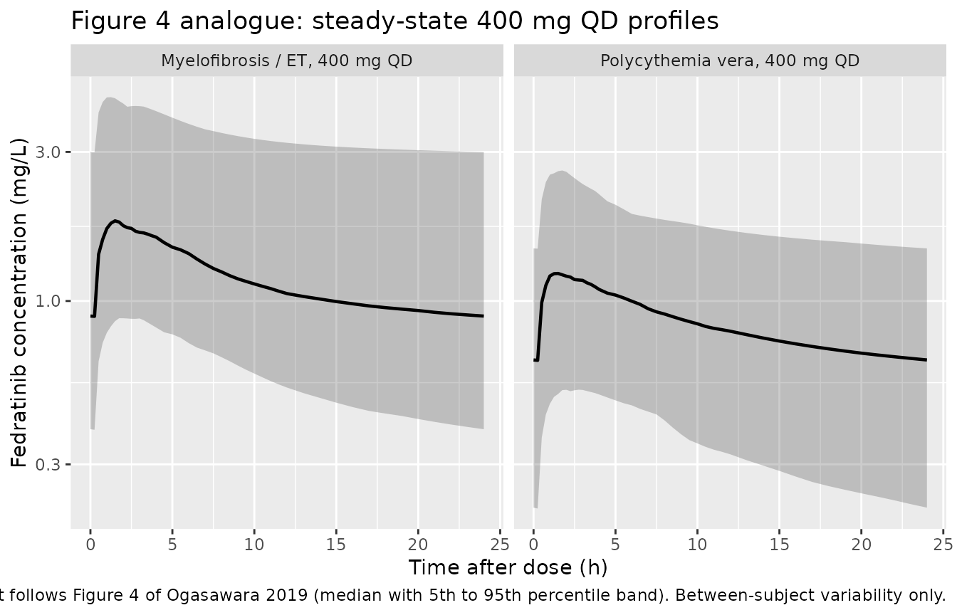
Cc is the individual prediction; the plots below
therefore display between-subject variability only. The log-additive
residual (expSd = 0.448 on the log scale) is not layered
on, so the simulated percentile band is narrower than the observed band
in the paper’s Figure 4.
Replicate published figures
Figure 1c and 1d: CL/F and V2/F by disease status
Figure 1c and 1d plot individual CL/F and V2/F from the base model by disease status at the 400 mg dose, with base-model typical values of 13.6 L/h and 340 L shown as dashed reference lines. The panels below are the final-model analogue.
per_subject <- sim |>
  dplyr::group_by(id, arm) |>
  dplyr::summarise(cl = dplyr::first(cl), vc = dplyr::first(vc), .groups = "drop")

per_subject |>
  tidyr::pivot_longer(c(cl, vc), names_to = "param", values_to = "value") |>
  dplyr::mutate(
    param = factor(
      param,
      levels = c("cl", "vc"),
      labels = c("CL/F (L/h)", "V2/F (L)")
    )
  ) |>
  ggplot(aes(arm, value)) +
  geom_boxplot(outlier.alpha = 0.3) +
  facet_wrap(~param, scales = "free_y") +
  scale_y_log10() +
  labs(
    x = NULL, y = NULL,
    title = "Figure 1c/1d analogue: CL/F and V2/F by disease status",
    caption = "Replicates the layout of Figure 1c and 1d of Ogasawara 2019, using the final model."
  ) +
  theme(axis.text.x = element_text(angle = 15, hjust = 1))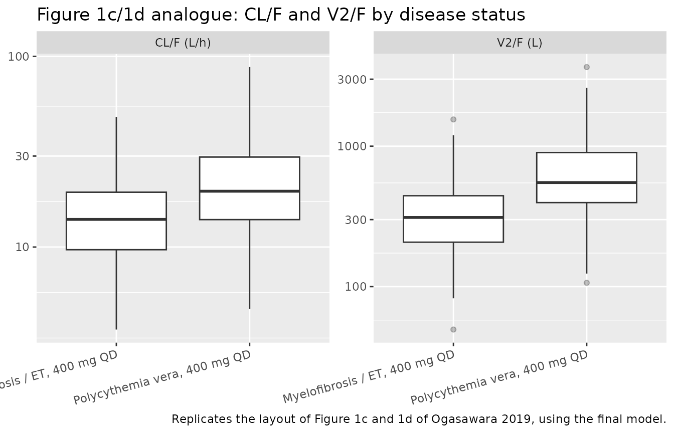
med <- per_subject |>
  dplyr::group_by(arm) |>
  dplyr::summarise(cl = median(cl), vc = median(vc), .groups = "drop")

cl_ratio <- med$cl[med$arm == "Polycythemia vera, 400 mg QD"] /
  med$cl[med$arm == "Myelofibrosis / ET, 400 mg QD"]
vc_ratio <- med$vc[med$arm == "Polycythemia vera, 400 mg QD"] /
  med$vc[med$arm == "Myelofibrosis / ET, 400 mg QD"]

# Cohort medians, so these are sampled quantities: the tolerance admits the
# sampling noise of a 150-per-arm draw while still failing loudly on a
# mis-transcribed factor (1.54 vs 1.87, or either read as its reciprocal).
stopifnot(
  abs(cl_ratio - 1.54) < 0.25,
  abs(vc_ratio - 1.87) < 0.35
)
Figure 2: forest plot of the significant covariate effects
Figure 2 is a forest plot of the covariate effects with references myelofibrosis/ET (diagnosis), normal renal function (CLcr at least 90 mL/min), 400 mg (dose) and the second body-weight tertile. The point estimates below are computed directly from the Table 2 coefficients.
forest <- tibble::tribble(
  ~param, ~label, ~ratio,
  "CL/F", "Polycythemia vera vs MF/ET", 1.54,
  "CL/F", "CLcr 30 mL/min vs 90 mL/min", (30 / 90)^0.294,
  "CL/F", "CLcr 60 mL/min vs 90 mL/min", (60 / 90)^0.294,
  "V2/F", "Polycythemia vera vs MF/ET", 1.87,
  "V2/F", "Weight 39.5 kg vs 70.1 kg", (39.5 / 70.1)^0.727,
  "V2/F", "Weight 135 kg vs 70.1 kg", (135 / 70.1)^0.727,
  "V2/F", "Dose 100 mg vs 400 mg", (100 / 400)^-0.279,
  "V2/F", "Dose 800 mg vs 400 mg", (800 / 400)^-0.279
)

forest |>
  ggplot(aes(ratio, label)) +
  geom_vline(xintercept = 1, linetype = "dashed") +
  geom_point(size = 2.5) +
  facet_wrap(~param, scales = "free_y", ncol = 1) +
  scale_x_log10() +
  labs(
    x = "Ratio to reference", y = NULL,
    title = "Figure 2 analogue: covariate effects on CL/F and V2/F",
    caption = "Replicates Figure 2 of Ogasawara 2019 (point estimates only; the published plot adds 90% CIs)."
  )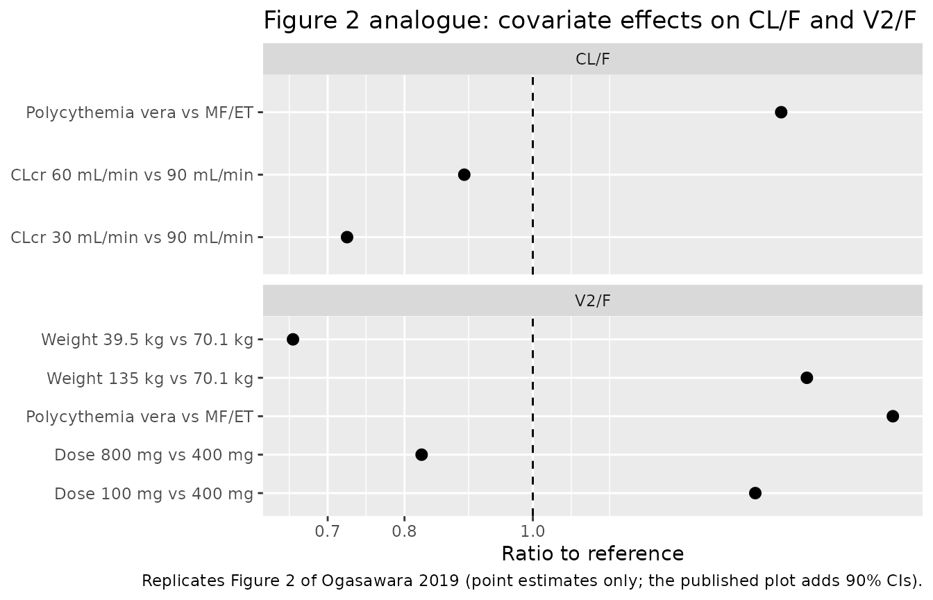
Figure 4: steady-state concentration-time profiles
sim |>
  dplyr::group_by(arm, time) |>
  dplyr::summarise(
    Q05 = quantile(Cc, 0.05),
    Q50 = quantile(Cc, 0.50),
    Q95 = quantile(Cc, 0.95),
    .groups = "drop"
  ) |>
  ggplot(aes(time, Q50)) +
  geom_ribbon(aes(ymin = Q05, ymax = Q95), alpha = 0.25) +
  geom_line(linewidth = 0.8) +
  facet_wrap(~arm) +
  scale_y_log10() +
  labs(
    x = "Time after dose (h)", y = "Fedratinib concentration (mg/L)",
    title = "Figure 4 analogue: steady-state 400 mg QD profiles",
    caption = paste(
      "Layout follows Figure 4 of Ogasawara 2019 (median with 5th to 95th",
      "percentile band). Between-subject variability only."
    )
  )
PKNCA validation
For a linear model, dose divided by AUC0-inf after a
single dose recovers CL/F exactly. That makes NCA on the typical-value
profile a direct, closed-form check on the whole solved system –
absorption, lag time, both disposition compartments and the covariate
model – against the published CL/F values of 13.0 L/h (MF/ET) and 20.0
L/h (PV).
The terminal half-life implied by Table 2 is long (the beta phase has a half-life near 114 h), so the profile is sampled out to 1000 h to characterise it.
nca_grid <- tidyr::expand_grid(
  DIS_PV = c(0, 1),
  DOSE = 400
) |>
  dplyr::mutate(
    id = dplyr::row_number(),
    WT = ref_wt,
    CRCL = ref_crcl,
    arm = ifelse(DIS_PV == 1, "Polycythemia vera", "Myelofibrosis / ET")
  )

nca_times <- sort(unique(c(
  seq(0, 12, by = 0.1), seq(12.5, 48, by = 0.5),
  seq(50, 240, by = 2), seq(244, 1000, by = 4)
)))

nca_ev <- nca_grid |>
  dplyr::mutate(time = 0, amt = DOSE, evid = 1L, cmt = "depot") |>
  dplyr::bind_rows(
    tidyr::expand_grid(nca_grid, time = nca_times) |>
      dplyr::mutate(amt = NA_real_, evid = 0L, cmt = "central")
  ) |>
  dplyr::arrange(id, time, dplyr::desc(evid)) |>
  dplyr::select(id, time, amt, evid, cmt, dplyr::everything())

nca_sim <- rxode2::rxSolve(mod_typ, events = nca_ev, keep = c("arm")) |>
  as.data.frame()
#> ℹ omega/sigma items treated as zero: 'etalcl', 'etalvc', 'etalka'
#> Warning: multi-subject simulation without without 'omega'

# Solver noise in the far tail can drive a decayed concentration slightly
# negative; PKNCA would then take log() of it and return NaN for aucinf.obs.
stopifnot(all(nca_sim$Cc >= 0))
sim_nca <- nca_sim |>
  dplyr::filter(!is.na(Cc)) |>
  dplyr::select(id, time, Cc, arm)

# Guarantee a time = 0 row per subject; pre-dose Cc = 0 is correct for an
# extravascular dose. Existing time = 0 rows win via .keep_all on the first
# occurrence.
sim_nca <- dplyr::bind_rows(
  sim_nca,
  sim_nca |> dplyr::distinct(id, arm) |> dplyr::mutate(time = 0, Cc = 0)
) |>
  dplyr::distinct(id, arm, time, .keep_all = TRUE) |>
  dplyr::arrange(id, arm, time)

dose_df <- nca_ev |>
  dplyr::filter(evid == 1L) |>
  dplyr::select(id, time, amt, arm)

conc_obj <- PKNCA::PKNCAconc(
  sim_nca, Cc ~ time | arm + id,
  concu = "mg/L", timeu = "h"
)
dose_obj <- PKNCA::PKNCAdose(dose_df, amt ~ time | arm + id, doseu = "mg")

intervals <- data.frame(
  start = 0, end = Inf,
  cmax = TRUE, tmax = TRUE, aucinf.obs = TRUE,
  half.life = TRUE, cl.obs = TRUE
)

nca_res <- PKNCA::pk.nca(PKNCA::PKNCAdata(conc_obj, dose_obj, intervals = intervals))
# The only NCA-comparable quantities Ogasawara 2019 publishes are the typical
# apparent clearances: 13.0 L/h for MF/ET (Table 2) and 20.0 L/h for a typical
# PV patient (Discussion). There is no published Cmax / Tmax / AUC table.
published <- tibble::tibble(
  arm = c("Myelofibrosis / ET", "Polycythemia vera"),
  cl.obs = c(13.0, 20.0)
)

cmp <- nlmixr2lib::ncaComparisonTable(
  simulated = nca_res,
  reference = published,
  by = "arm",
  params = "cl.obs",
  units = c(cl.obs = "L/h"),
  tolerance_pct = 20
)

knitr::kable(
  cmp,
  caption = paste(
    "Simulated vs published apparent clearance. Simulated CL/F is dose divided",
    "by PKNCA AUC0-inf on the typical-value 400 mg single-dose profile.",
    "* differs from reference by more than 20 per cent."
  )
)| NCA parameter | arm | Reference | Simulated | % diff |
|---|---|---|---|---|
| CL/F (L/h) | Myelofibrosis / ET | 13 | 13 | +0.1% |
| CL/F (L/h) | Polycythemia vera | 20 | 20 | +0.2% |
nca_tbl <- as.data.frame(nca_res$result) |>
  dplyr::filter(PPTESTCD %in% c("cmax", "tmax", "aucinf.obs", "half.life", "cl.obs")) |>
  dplyr::select(arm, PPTESTCD, PPORRES) |>
  tidyr::pivot_wider(names_from = PPTESTCD, values_from = PPORRES)

nca_tbl |>
  dplyr::select(arm, cmax, tmax, aucinf.obs, half.life) |>
  dplyr::rename(
    "Disease group" = arm,
    "Cmax (mg/L)" = cmax,
    "Tmax (h)" = tmax,
    "AUC0-inf (mg h/L)" = aucinf.obs,
    "t-half (h)" = half.life
  ) |>
  knitr::kable(
    digits = 3,
    caption = paste(
      "Remaining PKNCA parameters of the same typical-value profiles. These have",
      "no published counterpart in Ogasawara 2019 and are reported for context",
      "only, not as a validation gate. The long terminal half-life is the beta",
      "phase implied by V3/F = 1460 L against CL/F = 13.0 L/h."
    )
)| Disease group | Cmax (mg/L) | Tmax (h) | AUC0-inf (mg h/L) | t-half (h) |
|---|---|---|---|---|
| Myelofibrosis / ET | 0.967 | 1.8 | 30.747 | 113.154 |
| Polycythemia vera | 0.563 | 2.1 | 19.966 | 87.551 |
cl_nca <- setNames(nca_tbl$cl.obs, nca_tbl$arm)

# Typical-value (zeroRe) profiles, so the only error here is numerical
# (integration grid plus terminal extrapolation), not cohort sampling. A tight
# bound is therefore correct and is what makes this catch a transcription error.
stopifnot(
  abs(cl_nca[["Myelofibrosis / ET"]] / 13.0 - 1) < 0.02,
  abs(cl_nca[["Polycythemia vera"]] / 20.0 - 1) < 0.02,
  # The PV / MF ratio is the 1.54 factor recovered through the full solve.
  abs(cl_nca[["Polycythemia vera"]] / cl_nca[["Myelofibrosis / ET"]] - 1.54) < 0.02
)
Recovering both published clearances through a full solve is a strong
check: it exercises the absorption rate, the lag time, both disposition
compartments and the covariate model together, and it is sensitive to a
transcription error in any of lcl,
e_dis_pv_cl, e_crcl_cl, lq or
lvp.
Weight and dose: the two Discussion claims about Cmax and AUC
The Discussion makes two mechanistic claims that follow from weight and dose acting on V2/F but not on CL/F: Cmax increases in a slightly more than dose-proportional manner and is inversely correlated with body weight, while AUC is unaffected by weight. Both are checked on typical-value profiles.
claim_grid <- tidyr::expand_grid(
  DOSE = c(300, 400, 500),
  WT = c(50, 70.1, 100)
) |>
  dplyr::mutate(id = dplyr::row_number(), DIS_PV = 0, CRCL = ref_crcl)

claim_ev <- claim_grid |>
  dplyr::mutate(time = 0, amt = DOSE, evid = 1L, cmt = "depot") |>
  dplyr::bind_rows(
    # Tmax is near 1.5 h, so a fine grid over the first 12 h resolves Cmax.
    tidyr::expand_grid(claim_grid, time = seq(0, 12, by = 0.01)) |>
      dplyr::mutate(amt = NA_real_, evid = 0L, cmt = "central")
  ) |>
  dplyr::arrange(id, time, dplyr::desc(evid)) |>
  dplyr::select(id, time, amt, evid, cmt, dplyr::everything())

claim_sim <- rxode2::rxSolve(mod_typ, events = claim_ev) |>
  as.data.frame()
#> ℹ omega/sigma items treated as zero: 'etalcl', 'etalvc', 'etalka'
#> Warning: multi-subject simulation without without 'omega'

claim_sum <- claim_sim |>
  dplyr::group_by(id, DOSE, WT) |>
  dplyr::summarise(
    cl = dplyr::first(cl),
    vc = dplyr::first(vc),
    cmax = max(Cc),
    .groups = "drop"
  ) |>
  dplyr::mutate(
    cmax_per_mg = cmax / DOSE,
    # AUC0-inf of a linear model is exactly dose / CL, independent of every
    # volume term. Integrating the profile numerically would only add
    # truncation error to a quantity available in closed form.
    auc_inf = DOSE / cl
  )

knitr::kable(
  claim_sum |>
    dplyr::select(DOSE, WT, cl, vc, cmax, cmax_per_mg, auc_inf) |>
    dplyr::rename(
      "Dose (mg)" = DOSE, "Weight (kg)" = WT, "CL/F (L/h)" = cl,
      "V2/F (L)" = vc, "Cmax (mg/L)" = cmax,
      "Cmax per mg (mg/L/mg)" = cmax_per_mg, "AUC0-inf (mg h/L)" = auc_inf
    ),
  digits = 5,
  caption = "Typical-value CL/F, V2/F, Cmax and AUC across dose and body weight."
)| Dose (mg) | Weight (kg) | CL/F (L/h) | V2/F (L) | Cmax (mg/L) | Cmax per mg (mg/L/mg) | AUC0-inf (mg h/L) |
|---|---|---|---|---|---|---|
| 300 | 50.0 | 13.00975 | 263.5922 | 0.82809 | 0.00276 | 23.05962 |
| 300 | 70.1 | 13.00975 | 336.9910 | 0.67961 | 0.00227 | 23.05962 |
| 300 | 100.0 | 13.00975 | 436.2961 | 0.54837 | 0.00183 | 23.05962 |
| 400 | 50.0 | 13.00975 | 243.2622 | 1.17603 | 0.00294 | 30.74616 |
| 400 | 70.1 | 13.00975 | 311.0000 | 0.96728 | 0.00242 | 30.74616 |
| 400 | 100.0 | 13.00975 | 402.6460 | 0.78212 | 0.00196 | 30.74616 |
| 500 | 50.0 | 13.00975 | 228.5792 | 1.54296 | 0.00309 | 38.43270 |
| 500 | 70.1 | 13.00975 | 292.2285 | 1.27130 | 0.00254 | 38.43270 |
| 500 | 100.0 | 13.00975 | 378.3428 | 1.02967 | 0.00206 | 38.43270 |
at_ref_wt <- claim_sum |> dplyr::filter(WT == 70.1) |> dplyr::arrange(DOSE)
at_ref_dose <- claim_sum |> dplyr::filter(DOSE == 400) |> dplyr::arrange(WT)

cmax_dose_ratio <- at_ref_wt$cmax_per_mg[3] / at_ref_wt$cmax_per_mg[1]

# Every quantity here is a typical-value (zeroRe) solve, so these are algebraic
# identities of the compiled model rather than statistics of a random cohort;
# exact tolerances are correct and are what make them catch a transcription
# error.
stopifnot(
  # EXACT gate on the two V2/F covariate coefficients, read back off the solve.
  max(abs(at_ref_wt$vc / (311 * (c(300, 400, 500) / 400)^-0.279) - 1)) < 1e-8,
  max(abs(
    at_ref_dose$vc / (311 * (c(50, 70.1, 100) / 70.1)^0.727 * 1) - 1
  )) < 1e-8,
  # EXACT gate on the Discussion's "does not affect AUC" claim: CL/F carries no
  # weight term, so AUC0-inf = dose / CL is bit-identical across weights.
  length(unique(signif(at_ref_dose$auc_inf, 12))) == 1L,
  # Cmax rises more than dose-proportionally.
  all(diff(at_ref_wt$cmax_per_mg) > 0),
  # ... but only slightly. The realised 300 -> 500 mg factor is BELOW the
  # (500/300)^0.279 = 1.153 that the V2/F dose exponent alone would predict,
  # because the same change in V2/F also raises kel = CL/V2 and k12 = Q/V2 and
  # so steepens the distribution loss during absorption. The window below is
  # wide enough to cover that second-order effect and still goes red if the
  # exponent's sign flips (ratio < 1) or its magnitude is mis-transcribed.
  cmax_dose_ratio > 1.05, cmax_dose_ratio < 1.25,
  # Cmax inversely correlated with body weight.
  all(diff(at_ref_dose$cmax) < 0)
)

cat(sprintf(
  "Dose-normalised Cmax rises by a factor of %.4f from 300 to 500 mg (the V2/F dose exponent alone predicts %.4f).\n",
  cmax_dose_ratio, (500 / 300)^0.279
))
#> Dose-normalised Cmax rises by a factor of 1.1224 from 300 to 500 mg (the V2/F dose exponent alone predicts 1.1532).
The monotonicity and exact-equality assertions above are legitimate
despite being sign / equality claims on simulated quantities: these are
typical-value (zeroRe) solves, so the profiles differ only
by the covariate model, not by a random draw. The same assertions on the
stochastic cohort would not be safe.
Assumptions and deviations
- CLcr normalisation constant. Table 2 footnote b normalises CLcr at 78.3 mL/min while Table 1 reports the cohort median as 78.5 mL/min. The printed equation governs, so the model uses 78.3. The discrepancy changes CL/F by 0.075 per cent at the median and is invisible in every check above; the Discussion’s “typical PV patient (CLcr = 78.5 mL/min) was 20.0 L/h” rounds to 20.0 under either reading and so does not arbitrate between them.
-
Study identifier. The Methods name the fifth study
ARD12888(NCT01692366); Supplementary Table 1 names the same studyARD12188. The subject and sample counts reconcile exactly (52 + 31 + 78 + 97 + 8 + 186 = 452 subjects; 621 + 516 + 1206 + 511 + 97 + 491 = 3442 samples), so this is a typographical inconsistency in the source, not a missing study. The model metadata uses the Supplementary Table 1 spelling. -
Residual error encoding. The Methods state that
concentrations were natural-log transformed and that residual
variability was additive. That is log-normal residual error in linear
space, encoded as
Cc ~ lnorm(expSd)withexpSd = sqrt(0.201) = 0.448. It is not encoded as a proportional error: at this magnitude the two are not interchangeable. -
Dose as a covariate.
DOSEenters V2/F as a data column and must be supplied alongside theamtof the dose records. The final model was fit to doses of 100 mg and above; the authors deliberately excluded the 30 to 60 mg data because CL/F and V2/F were dose-dependent below about 120 mg. The packaged model applies(DOSE/400)^-0.279without a clamp, exactly as printed, so extrapolation below 100 mg is outside the model’s validated range. - Covariate distributions. Body weight and creatinine clearance are drawn as truncated log-normals matched to the Table 1 medians and ranges. The paper publishes no correlation structure between them, so they are drawn independently; the real cohort almost certainly has a weight/CLcr correlation through the Cockcroft-Gault formula.
-
Race, sex, age and hepatic function are not in the
model. They were screened and found not clinically meaningful
(Discussion), and are recorded in the model file’s
covariatesDataExcludedrather thancovariateData. -
Residual error is excluded from the VPC figure. The
Figure 4 analogue plots percentiles of
Cc(the individual prediction), so its band reflects between-subject variability only and is narrower than the paper’s prediction-corrected VPC of observed data. - No IIV on the lag time or on Q/F and V3/F. The paper states interindividual variability was determined for CL/F, V2/F and ka only, so no other random effects are declared.
-
Bioavailability is not a parameter. All clearances
and volumes are apparent (
/F) values; F is implicitly 1 and nolfdepotis declared. -
No non-paper-derived parameter values. Every
ini()entry traces to Table 2 of Ogasawara 2019.