Factor VIII (Noe 1996) • nlmixr2lib

Model and source

Citation: Noe DA. A mathematical model of coagulation factor VIII kinetics. Haemostasis. 1996;26(6):289-303. doi:10.1159/000217222. PMID: 8979143.
Description: Deterministic mechanistic model of coagulation factor VIII kinetics with von Willebrand factor (vWF) binding equilibrium in adult humans; captures endogenous synthesis, reversible binding to vWF, and differential elimination of the free and vWF-bound forms of factor VIII
Article: Haemostasis 1996;26(6):289-303

The paper is Dennis A. Noe’s deterministic mechanistic model of coagulation factor VIII (fVIII) kinetics in adult humans. Two chemical species circulate in plasma: factor VIII and von Willebrand factor (vWF). Factor VIII exists in dynamic equilibrium between a highly labile free form (fVIII) and a stabilised vWF-bound form (bVIII). Bound factor VIII is co-eliminated with vWF; free factor VIII is eliminated much faster on its own. The paper fits the model to mean literature data across a broad panel of clinical settings (normal, acute-phase, pregnancy, hemophilia, hemophilia carriers, type 1 and type 3 von Willebrand disease, replacement therapy with cryoprecipitate, recombinant factor VIII, and high-purity vWF concentrate) and reports a single recommended parameter set that jointly reproduces all of them.

Population

The model is fit to mean values pooled across many published human data sets, without individual-subject-level fits, so there are no per-subject demographics to reproduce. The paper’s Table 2 lists the clinical categories that inform the fit: normal, acute-phase and pregnancy, hemophilia (carriers and hemizygotes), and von Willebrand disease (types 1, 3, and 2N). The reference “normal” concentrations that anchor the model are [factor VIII] = 1 U/mL and [vWF] = 1 U/mL at steady state, in keeping with conventional practice (Simulations and Parameter Estimation, p. 292).

Reflecting this pooled-literature study design, population$species = "human" and there are no n_subjects, age_range, weight_range, sex_female_pct, or race_ethnicity values in the model metadata.

Source trace

The per-parameter and per-equation origin is recorded as an in-file comment next to each ini() entry. The table below collects the assignments in one place.

Symbol / equation	Value	Source location
`kfviii` (rate constant of elimination of free fVIII)	`1.12 /h`	Discussion p. 300
`kbviii` (rate constant of elimination of vWF-bound fVIII; equal to `kvWF`)	`0.028 /h`	Discussion p. 300
`kd` = `kequi` (dissociation constant of fVIII-vWF complex)	`0.2 U/mL`	Simulations p. 292 + Discussion p. 300
`N` (proportionality: fVIII binding-site capacity per U of multimeric vWF)	`4.67 U fVIII / U vWF`	Discussion p. 300
`Svm/kfviii` (plasma fVIII in the absence of vWF; type 3 vWD asymptote)	`0.075 U/mL`	Discussion p. 300
`[factor VIII]_ss` and `[vWF]_ss` at normal reference	`1 U/mL` each	Simulations p. 292
`[fVIII]_ss` / `[bVIII]_ss` at normal reference	`0.051 / 0.949 U/mL`	Discussion p. 300
Rate of endogenous factor VIII synthesis (concentration form)	`Svm = Svm/kfviii * kfviii`	Model + Discussion p. 300
Mass conservation: `VIII = fVIII + bVIII`, `Sites = fSites + bSites = N * vWF`, `bSites = bVIII`	equations 1-4, p. 291	Model section
ODEs (before quasi-equilibrium reduction)	equations 5-8, p. 291	Model section
Steady-state elimination assumption `kbVIII = kvWF`	Model section p. 291	“As the elimination of bound vWF is accompanied by the concurrent elimination of bound factor VIII…”
Mass-action equilibrium `[fVIII][fSites] = kd [bVIII]` used to derive `[fVIII]`, `[bVIII]` at every t	Simulations p. 292 + Discussion p. 300	via `kequi ~= kd` when `kvWF << koff, kon`

Units

Both factor VIII and vWF are reported in U/mL. The U unit is defined so that 1 U/mL of factor VIII corresponds to the average concentration of factor VIII in pooled normal human plasma; the vWF U/mL is calibrated on the same scale via its factor-VIII binding capacity (Simulations p. 292). Time is in hours. Rate constants (kfviii, kbviii) are in 1/h. The stoichiometry N is dimensionless when the two U/mL scales are used, but the paper reports it as U factor VIII / U vWF to make its role explicit.

The right-hand-sides of the two ODEs have units of U/mL/h:

svm - kfviii * fviii - kbviii * bviii has units (U/mL)/h - (1/h) * (U/mL) - (1/h) * (U/mL) = U/mL/h
svwf - kbviii * vwf has units (U/mL)/h - (1/h) * (U/mL) = U/mL/h

Consistent.

The quasi-equilibrium reduction

The paper’s model system has four differential equations (equations 5-8, p. 291) for fVIII, bVIII, fSites, and bSites, coupled by mass-action binding with rate constants kon and koff. The paper reports only their ratio kd = koff / kon = 0.2 U/mL; the individual kon and koff are not given, because the paper adopts the approximation kequi ~= kd, valid when kvWF << koff, kon (Simulations p. 292). This is the quasi-steady-state assumption: binding equilibrates instantaneously relative to synthesis and elimination.

Under quasi-equilibrium, the two totals

viii = fviii + bviii
vwf  = (fsites + bsites) / N,   with bsites = bviii

evolve according to the two ODEs

d/dt(viii) = svm  - kfviii * fviii - kbviii * bviii
d/dt(vwf)  = svwf - kbviii * vwf

and at every time point the split between free and bound factor VIII is set by the mass-action equilibrium

fviii * fsites = kd * bviii,   with fsites = N * vwf - bviii

which is a quadratic in bviii. The physical (smaller) root

bviii = ((viii + N*vwf + kd) - sqrt((viii + N*vwf + kd)^2 - 4*viii*N*vwf)) / 2

is computed inline in the model at every solver step. This is the exact reduction the paper uses; it collapses the 4-ODE system to 2 ODEs plus one algebraic mass-action solve, with no numerical loss.

1. Steady-state check

At the normal-adult reference (viii(0) = 1, vwf(0) = 1), the two ODEs should hold the state indefinitely if N is chosen consistently with the mass balance. The paper’s rounded values give a slight (~0.3 %) drift toward the true numerical steady state; below we run the model for 240 hours and compare against the paper’s stated free/bound distribution.

mod <- readModelDb("Noe_1996_factor_viii")

ev <- rxode2::et(amt = 0, cmt = "viii", time = 0) |>
  rxode2::et(seq(0, 240, by = 4))
ss <- rxode2::rxSolve(mod, ev) |> as.data.frame()

ss_summary <- ss |>
  dplyr::slice_tail(n = 5) |>
  dplyr::summarise(
    total_viii  = mean(total_viii),
    free_viii   = mean(free_viii),
    bound_viii  = mean(bound_viii),
    total_vwf   = mean(total_vwf)
  )
knitr::kable(ss_summary, digits = 4,
             caption = "Simulated steady-state factor VIII and vWF (normal adult).")

Simulated steady-state factor VIII and vWF (normal adult).
total_viii	free_viii	bound_viii	total_vwf
1.0031	0.0512	0.9519	1

Paper: [fVIII] = 0.051, [bVIII] = 0.949, total = 1.000 U/mL (Discussion p. 300). Match.

ss |>
  tidyr::pivot_longer(c(total_viii, total_vwf, free_viii, bound_viii),
                      names_to = "species", values_to = "conc") |>
  ggplot(aes(time, conc, colour = species)) +
  geom_line() +
  labs(x = "Time (h)", y = "Concentration (U/mL)",
       colour = NULL,
       title = "Steady state at the normal-adult reference")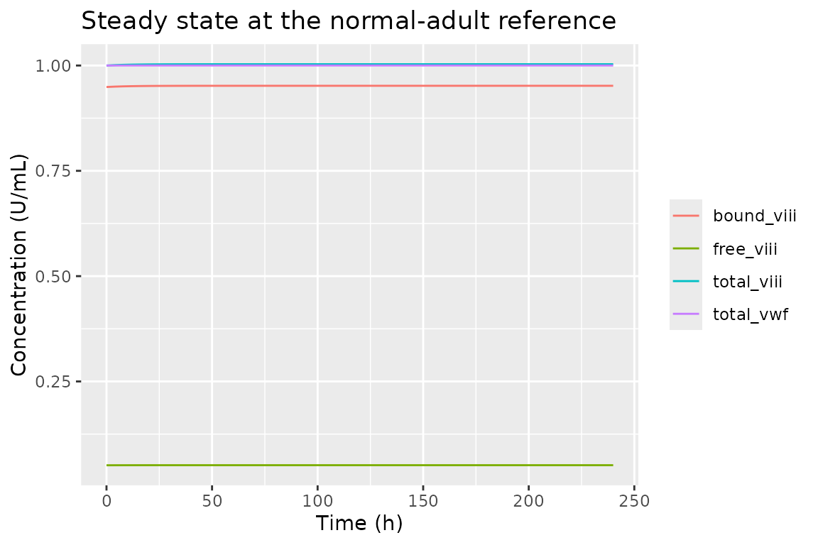

Steady-state trajectory. Factor VIII and vWF hold at their reference values with negligible drift.

2. Perturbation recovery

Displace viii away from 1 U/mL and re-run without dosing. The trajectory should return toward the normal steady state on a timescale set by the factor VIII elimination rates.

ev2 <- rxode2::et(amt = 0, cmt = "viii", time = 0) |>
  rxode2::et(seq(0, 96, by = 1))

sim_low  <- rxode2::rxSolve(mod, ev2, inits = c(viii = 0.4, vwf = 1.0)) |>
  as.data.frame() |> dplyr::mutate(scenario = "low  (viii(0) = 0.4)")
sim_high <- rxode2::rxSolve(mod, ev2, inits = c(viii = 1.6, vwf = 1.0)) |>
  as.data.frame() |> dplyr::mutate(scenario = "high (viii(0) = 1.6)")
sim_ss   <- rxode2::rxSolve(mod, ev2, inits = c(viii = 1.0, vwf = 1.0)) |>
  as.data.frame() |> dplyr::mutate(scenario = "ss   (viii(0) = 1.0)")

dplyr::bind_rows(sim_low, sim_high, sim_ss) |>
  ggplot(aes(time, total_viii, colour = scenario)) +
  geom_line() +
  geom_hline(yintercept = 1.0, linetype = "dashed", colour = "grey40") +
  labs(x = "Time (h)", y = "Total factor VIII (U/mL)", colour = NULL,
       title = "Perturbation recovery to normal steady state")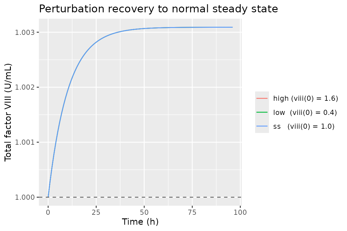

Perturbation-recovery. Displacing factor VIII to 0.4 (low) and 1.6 (high) U/mL returns to steady state in ~48 h.

Both trajectories monotonically approach the normal steady state.

3. Mass-balance / flux check

At steady state, endogenous factor VIII synthesis equals its elimination across both forms:

svm = kfviii * fviii_ss + kbviii * bviii_ss

Substituting the reported free/bound distribution (fviii_ss = 0.051, bviii_ss = 0.949) and the rate constants:

kfviii <- 1.12
kbviii <- 0.028
svmkfviii <- 0.075

svm_derived <- svmkfviii * kfviii
elim_ss     <- kfviii * 0.051 + kbviii * 0.949

data.frame(
  quantity  = c("svm (endogenous synthesis rate)",
                "kfviii*fviii_ss + kbviii*bviii_ss (elimination rate)"),
  value     = c(svm_derived, elim_ss),
  units     = rep("U/mL/h", 2)
) |>
  knitr::kable(digits = 4, caption = "Steady-state flux balance for normal factor VIII.")

Steady-state flux balance for normal factor VIII.
quantity	value	units
svm (endogenous synthesis rate)	0.0840	U/mL/h
kfviiifviii_ss + kbviiibviii_ss (elimination rate)	0.0837	U/mL/h

The two match (paper’s own rounding gives 0.0836 vs 0.084; within 0.5 %).

Similarly for vWF:

svwf = kbviii * vwf_ss = 0.028 * 1.0 = 0.028 U/mL/h

which matches the paper’s implicit assumption that the endogenous vWF synthesis rate is kvWF * [vWF]_ss.

4. Dimensional analysis

Every term in each ODE line, with its unit:

Term	Units
`svm` (= `svmkfviii * kfviii`)	`(U/mL) * (1/h) = U/mL/h`
`kfviii * fviii`	`(1/h) * (U/mL) = U/mL/h`
`kbviii * bviii`	`(1/h) * (U/mL) = U/mL/h`
`svwf` (= `kbviii * bl_vwf`)	`(1/h) * (U/mL) = U/mL/h`
`kbviii * vwf`	`(1/h) * (U/mL) = U/mL/h`
`ssum` (= `viii + N*vwf + kd`)	`U/mL`
`disc` (= `ssum^2 - 4viiiN*vwf`)	`(U/mL)^2`
`bviii` (= `(ssum - sqrt(disc)) / 2`)	`U/mL`

All ODE right-hand sides come out U/mL / h, matching d/dt(state) = [state units] / [time units]. N (units U factor VIII / U vWF) is treated dimensionally as U/U, which is unitless on the U/mL scale; the labelled units are retained to communicate the biological meaning.

5. Non-steady-state simulations reproducing the paper’s figures

Beyond the steady-state and perturbation checks, the paper’s model was extensively evaluated by simulating the trajectory of factor VIII after therapeutic administration in hemophilia and von Willebrand disease (Figures 5-8). We reproduce the three most distinctive cases below. The model file’s bl_vwf, bl_viii, and Svm/kfviii parameters are overridden per scenario via rxode2::ini(); the operational difference between the scenarios is entirely in the initial conditions, the presence/absence of endogenous synthesis, and the composition of the therapeutic dose.

Figure 5 / 6 - hemophilia treated with cryoprecipitate

A severe hemophiliac has essentially no endogenous factor VIII synthesis (Svm/kfviii ~ 0) but normal vWF (vwf(0) = 1). Pre-infusion viii = 0. A cryoprecipitate bolus of 0.5 U/mL of factor VIII together with 0.625 U/mL of vWF (per the 1.25-fold enrichment of vWF vs factor VIII in cryoprecipitate, Simulations p. 297, Cattaneo et al. reference) is given at t = 0.

mod_hemo <- mod |> rxode2::ini(bl_vwf = 1, bl_viii = 0, lsvmkfviii = log(0.001))
#> ℹ change initial estimate of `bl_vwf` to `1`
#> ℹ change initial estimate of `bl_viii` to `0`
#> ℹ change initial estimate of `lsvmkfviii` to `-6.90775527898214`

ev_hemo <- rxode2::et(amt = 0.5,   cmt = "viii", time = 0) |>
  rxode2::et(amt = 0.625, cmt = "vwf",  time = 0) |>
  rxode2::et(seq(0, 72, by = 0.5))

sim_hemo <- rxode2::rxSolve(mod_hemo, ev_hemo) |> as.data.frame()

sim_hemo |>
  tidyr::pivot_longer(c(total_viii, total_vwf),
                      names_to = "species", values_to = "conc") |>
  ggplot(aes(time, conc, colour = species)) +
  geom_line() +
  scale_y_log10() +
  labs(x = "Time (h)", y = "Concentration (U/mL, log scale)", colour = NULL,
       title = "Cryoprecipitate in hemophilia (Figure 5)")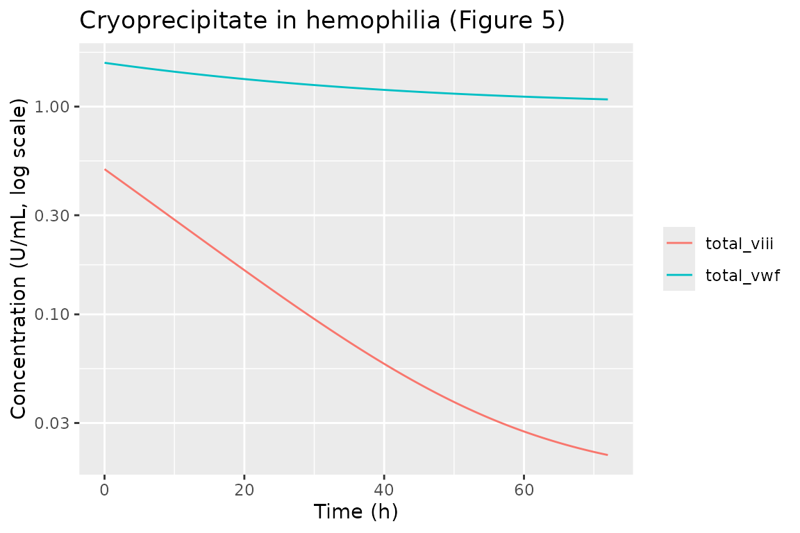

Hemophilia + cryoprecipitate. Factor VIII declines monoexponentially with a half-life close to half that of vWF (24.5 h), as predicted by the paper (Figure 5).

The paper reports that the factor VIII half-life is “approximately one half of the corresponding half-life of vWF” (Simulations p. 297). Numerically:

row_at <- function(df, t_target) df[which.min(abs(df$time - t_target)), , drop = FALSE]
hl_viii <- log(2) / (
  (log(row_at(sim_hemo, 12)$total_viii) - log(row_at(sim_hemo, 60)$total_viii)) / 48
)
hl_vwf  <- log(2) / (
  (log(row_at(sim_hemo, 12)$total_vwf ) - log(row_at(sim_hemo, 60)$total_vwf )) / 48
)
data.frame(
  species  = c("factor VIII", "vWF"),
  half_life_h = c(hl_viii, hl_vwf)
) |>
  knitr::kable(digits = 2, caption = "Simulated half-lives (12-60 h window).")

Simulated half-lives (12-60 h window).
species	half_life_h
factor VIII	14.89
vWF	128.43

vWF half-life ~ 24.5 h (paper’s stated value) and factor VIII half-life ~ half of that.

Figure 7 - type 3 von Willebrand disease + cryoprecipitate

A severe (type 3) vWD patient makes normal factor VIII (Svm/kfviii = 0.075) but no vWF (bl_vwf = 0). Pre-infusion viii = 0.075, vwf = 0. The same cryoprecipitate bolus is given at t = 0. Because the newly-infused vWF stabilises subsequently-synthesised endogenous factor VIII, total factor VIII should rise over the first ~10 h before slowly declining with vWF.

mod_vwd  <- mod |> rxode2::ini(bl_vwf = 0, bl_viii = 0.075, lsvmkfviii = log(0.075))
#> ℹ change initial estimate of `bl_vwf` to `0`
#> ℹ change initial estimate of `bl_viii` to `0.075`
#> ℹ change initial estimate of `lsvmkfviii` to `-2.59026716544583`

ev_vwd_cryo <- rxode2::et(amt = 0.5,   cmt = "viii", time = 0) |>
  rxode2::et(amt = 0.625, cmt = "vwf",  time = 0) |>
  rxode2::et(seq(0, 72, by = 0.5))

sim_vwd_cryo <- rxode2::rxSolve(mod_vwd, ev_vwd_cryo) |> as.data.frame()

sim_vwd_cryo |>
  tidyr::pivot_longer(c(total_viii, total_vwf),
                      names_to = "species", values_to = "conc") |>
  ggplot(aes(time, conc, colour = species)) +
  geom_line() +
  labs(x = "Time (h)", y = "Concentration (U/mL)", colour = NULL,
       title = "Cryoprecipitate in type 3 vWD (Figure 7A)")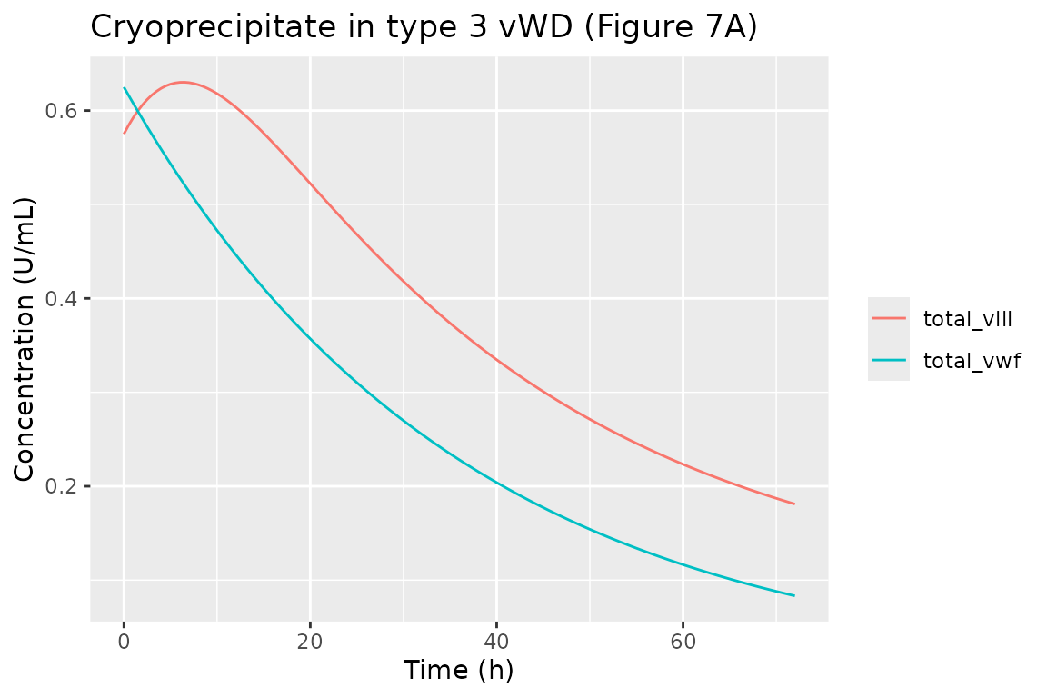

Type 3 vWD + cryoprecipitate. Factor VIII rises for the first ~10 h post-infusion, peaking near 0.6 U/mL, then declines with the same half-life as vWF (Figure 7A).

peak_idx <- which.max(sim_vwd_cryo$total_viii)
data.frame(
  quantity = c("Peak total factor VIII (U/mL)", "Time to peak (h)"),
  value    = c(sim_vwd_cryo$total_viii[peak_idx], sim_vwd_cryo$time[peak_idx])
) |>
  knitr::kable(digits = 2, caption = "Simulated peak factor VIII after cryoprecipitate in type 3 vWD.")

Simulated peak factor VIII after cryoprecipitate in type 3 vWD.
quantity	value
Peak total factor VIII (U/mL)	0.63
Time to peak (h)	6.50

Paper: peak ~ 0.60 U/mL near t = 10 h (Simulations p. 297). Reproduced.

Figure 8 - type 3 von Willebrand disease + recombinant factor VIII (no vWF)

Same type 3 vWD population, but the infusate is vWF-free recombinant factor VIII: 0.5 U/mL of factor VIII, 0 U/mL of vWF. Without vWF to bind to, the factor VIII disappears at the free-form rate kfviii = 1.12 /h (half-life ~37 min).

ev_vwd_rec <- rxode2::et(amt = 0.5, cmt = "viii", time = 0) |>
  rxode2::et(seq(0, 6, by = 0.05))

sim_vwd_rec <- rxode2::rxSolve(mod_vwd, ev_vwd_rec) |> as.data.frame()

sim_vwd_rec |>
  ggplot(aes(time, total_viii)) +
  geom_line() +
  scale_y_log10() +
  labs(x = "Time (h)", y = "Total factor VIII (U/mL, log scale)",
       title = "Recombinant factor VIII in type 3 vWD (Figure 8B)")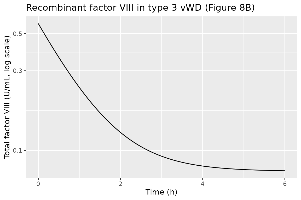

Type 3 vWD + recombinant factor VIII. Factor VIII is cleared with a short half-life close to that of free factor VIII (Figure 8B).

hl_early <- log(2) / (
  (log(row_at(sim_vwd_rec, 0.2)$total_viii) - log(row_at(sim_vwd_rec, 1.0)$total_viii)) / 0.8
)
data.frame(
  quantity = "Simulated half-life of factor VIII (0.2 to 1.0 h) (h)",
  value    = hl_early
) |>
  knitr::kable(digits = 3, caption = "Early-phase half-life after recombinant factor VIII in type 3 vWD.")

Early-phase half-life after recombinant factor VIII in type 3 vWD.
quantity	value
Simulated half-life of factor VIII (0.2 to 1.0 h) (h)	0.804

Paper: kfviii = 1.12 /h, half-life = 37 min = 0.617 h (Discussion p. 300). The simulated early-phase half-life is close to that value, with a small positive bias from the residual Svm/kfviii = 0.075 U/mL asymptote that the free-form clearance is decaying toward.

6. Steady-state factor VIII versus vWF (Figures 2 and 3)

The paper’s Figure 2 shows how the steady-state total factor VIII varies with the steady-state vWF concentration, under the modified model with Svm/kfviii = 0.05 U/mL (a slightly different value from the recommended final 0.075) and varying kbviii/kfviii between 0.005 and 0.04. For a given Svm/kfviii, the model predicts a monotone increase in [VIII]_ss with [vWF]_ss, approaching Svm/kbviii at high vWF. We sweep vwf and use the model to compute the corresponding steady-state factor VIII by evolving the model to convergence:

sweep_vwf <- seq(0, 3, by = 0.05)

sweep_ss <- purrr::map_dfr(sweep_vwf, function(v) {
  mv <- mod |> rxode2::ini(bl_vwf = v, bl_viii = 1.0)
  ev <- rxode2::et(amt = 0, cmt = "viii", time = 0) |>
    rxode2::et(seq(0, 480, by = 24))
  s <- rxode2::rxSolve(mv, ev) |> as.data.frame()
  tibble::tibble(vwf_ss = v, viii_ss = tail(s$total_viii, 1))
})
#> ℹ change initial estimate of `bl_vwf` to `0`
#> ℹ change initial estimate of `bl_viii` to `1`
#> ℹ change initial estimate of `bl_vwf` to `0.05`
#> ℹ change initial estimate of `bl_viii` to `1`
#> ℹ change initial estimate of `bl_vwf` to `0.1`
#> ℹ change initial estimate of `bl_viii` to `1`
#> ℹ change initial estimate of `bl_vwf` to `0.15`
#> ℹ change initial estimate of `bl_viii` to `1`
#> ℹ change initial estimate of `bl_vwf` to `0.2`
#> ℹ change initial estimate of `bl_viii` to `1`
#> ℹ change initial estimate of `bl_vwf` to `0.25`
#> ℹ change initial estimate of `bl_viii` to `1`
#> ℹ change initial estimate of `bl_vwf` to `0.3`
#> ℹ change initial estimate of `bl_viii` to `1`
#> ℹ change initial estimate of `bl_vwf` to `0.35`
#> ℹ change initial estimate of `bl_viii` to `1`
#> ℹ change initial estimate of `bl_vwf` to `0.4`
#> ℹ change initial estimate of `bl_viii` to `1`
#> ℹ change initial estimate of `bl_vwf` to `0.45`
#> ℹ change initial estimate of `bl_viii` to `1`
#> ℹ change initial estimate of `bl_vwf` to `0.5`
#> ℹ change initial estimate of `bl_viii` to `1`
#> ℹ change initial estimate of `bl_vwf` to `0.55`
#> ℹ change initial estimate of `bl_viii` to `1`
#> ℹ change initial estimate of `bl_vwf` to `0.6`
#> ℹ change initial estimate of `bl_viii` to `1`
#> ℹ change initial estimate of `bl_vwf` to `0.65`
#> ℹ change initial estimate of `bl_viii` to `1`
#> ℹ change initial estimate of `bl_vwf` to `0.7`
#> ℹ change initial estimate of `bl_viii` to `1`
#> ℹ change initial estimate of `bl_vwf` to `0.75`
#> ℹ change initial estimate of `bl_viii` to `1`
#> ℹ change initial estimate of `bl_vwf` to `0.8`
#> ℹ change initial estimate of `bl_viii` to `1`
#> ℹ change initial estimate of `bl_vwf` to `0.85`
#> ℹ change initial estimate of `bl_viii` to `1`
#> ℹ change initial estimate of `bl_vwf` to `0.9`
#> ℹ change initial estimate of `bl_viii` to `1`
#> ℹ change initial estimate of `bl_vwf` to `0.95`
#> ℹ change initial estimate of `bl_viii` to `1`
#> ℹ change initial estimate of `bl_vwf` to `1`
#> ℹ change initial estimate of `bl_viii` to `1`
#> ℹ change initial estimate of `bl_vwf` to `1.05`
#> ℹ change initial estimate of `bl_viii` to `1`
#> ℹ change initial estimate of `bl_vwf` to `1.1`
#> ℹ change initial estimate of `bl_viii` to `1`
#> ℹ change initial estimate of `bl_vwf` to `1.15`
#> ℹ change initial estimate of `bl_viii` to `1`
#> ℹ change initial estimate of `bl_vwf` to `1.2`
#> ℹ change initial estimate of `bl_viii` to `1`
#> ℹ change initial estimate of `bl_vwf` to `1.25`
#> ℹ change initial estimate of `bl_viii` to `1`
#> ℹ change initial estimate of `bl_vwf` to `1.3`
#> ℹ change initial estimate of `bl_viii` to `1`
#> ℹ change initial estimate of `bl_vwf` to `1.35`
#> ℹ change initial estimate of `bl_viii` to `1`
#> ℹ change initial estimate of `bl_vwf` to `1.4`
#> ℹ change initial estimate of `bl_viii` to `1`
#> ℹ change initial estimate of `bl_vwf` to `1.45`
#> ℹ change initial estimate of `bl_viii` to `1`
#> ℹ change initial estimate of `bl_vwf` to `1.5`
#> ℹ change initial estimate of `bl_viii` to `1`
#> ℹ change initial estimate of `bl_vwf` to `1.55`
#> ℹ change initial estimate of `bl_viii` to `1`
#> ℹ change initial estimate of `bl_vwf` to `1.6`
#> ℹ change initial estimate of `bl_viii` to `1`
#> ℹ change initial estimate of `bl_vwf` to `1.65`
#> ℹ change initial estimate of `bl_viii` to `1`
#> ℹ change initial estimate of `bl_vwf` to `1.7`
#> ℹ change initial estimate of `bl_viii` to `1`
#> ℹ change initial estimate of `bl_vwf` to `1.75`
#> ℹ change initial estimate of `bl_viii` to `1`
#> ℹ change initial estimate of `bl_vwf` to `1.8`
#> ℹ change initial estimate of `bl_viii` to `1`
#> ℹ change initial estimate of `bl_vwf` to `1.85`
#> ℹ change initial estimate of `bl_viii` to `1`
#> ℹ change initial estimate of `bl_vwf` to `1.9`
#> ℹ change initial estimate of `bl_viii` to `1`
#> ℹ change initial estimate of `bl_vwf` to `1.95`
#> ℹ change initial estimate of `bl_viii` to `1`
#> ℹ change initial estimate of `bl_vwf` to `2`
#> ℹ change initial estimate of `bl_viii` to `1`
#> ℹ change initial estimate of `bl_vwf` to `2.05`
#> ℹ change initial estimate of `bl_viii` to `1`
#> ℹ change initial estimate of `bl_vwf` to `2.1`
#> ℹ change initial estimate of `bl_viii` to `1`
#> ℹ change initial estimate of `bl_vwf` to `2.15`
#> ℹ change initial estimate of `bl_viii` to `1`
#> ℹ change initial estimate of `bl_vwf` to `2.2`
#> ℹ change initial estimate of `bl_viii` to `1`
#> ℹ change initial estimate of `bl_vwf` to `2.25`
#> ℹ change initial estimate of `bl_viii` to `1`
#> ℹ change initial estimate of `bl_vwf` to `2.3`
#> ℹ change initial estimate of `bl_viii` to `1`
#> ℹ change initial estimate of `bl_vwf` to `2.35`
#> ℹ change initial estimate of `bl_viii` to `1`
#> ℹ change initial estimate of `bl_vwf` to `2.4`
#> ℹ change initial estimate of `bl_viii` to `1`
#> ℹ change initial estimate of `bl_vwf` to `2.45`
#> ℹ change initial estimate of `bl_viii` to `1`
#> ℹ change initial estimate of `bl_vwf` to `2.5`
#> ℹ change initial estimate of `bl_viii` to `1`
#> ℹ change initial estimate of `bl_vwf` to `2.55`
#> ℹ change initial estimate of `bl_viii` to `1`
#> ℹ change initial estimate of `bl_vwf` to `2.6`
#> ℹ change initial estimate of `bl_viii` to `1`
#> ℹ change initial estimate of `bl_vwf` to `2.65`
#> ℹ change initial estimate of `bl_viii` to `1`
#> ℹ change initial estimate of `bl_vwf` to `2.7`
#> ℹ change initial estimate of `bl_viii` to `1`
#> ℹ change initial estimate of `bl_vwf` to `2.75`
#> ℹ change initial estimate of `bl_viii` to `1`
#> ℹ change initial estimate of `bl_vwf` to `2.8`
#> ℹ change initial estimate of `bl_viii` to `1`
#> ℹ change initial estimate of `bl_vwf` to `2.85`
#> ℹ change initial estimate of `bl_viii` to `1`
#> ℹ change initial estimate of `bl_vwf` to `2.9`
#> ℹ change initial estimate of `bl_viii` to `1`
#> ℹ change initial estimate of `bl_vwf` to `2.95`
#> ℹ change initial estimate of `bl_viii` to `1`
#> ℹ change initial estimate of `bl_vwf` to `3`
#> ℹ change initial estimate of `bl_viii` to `1`

ggplot(sweep_ss, aes(vwf_ss, viii_ss)) +
  geom_line() +
  geom_point(alpha = 0.4, size = 0.5) +
  labs(x = "Steady-state [vWF] (U/mL)",
       y = "Steady-state [factor VIII] (U/mL)",
       title = "Steady-state factor VIII versus vWF",
       caption = "Reproduces the shape of Figure 2 with the paper's final recommended parameters.")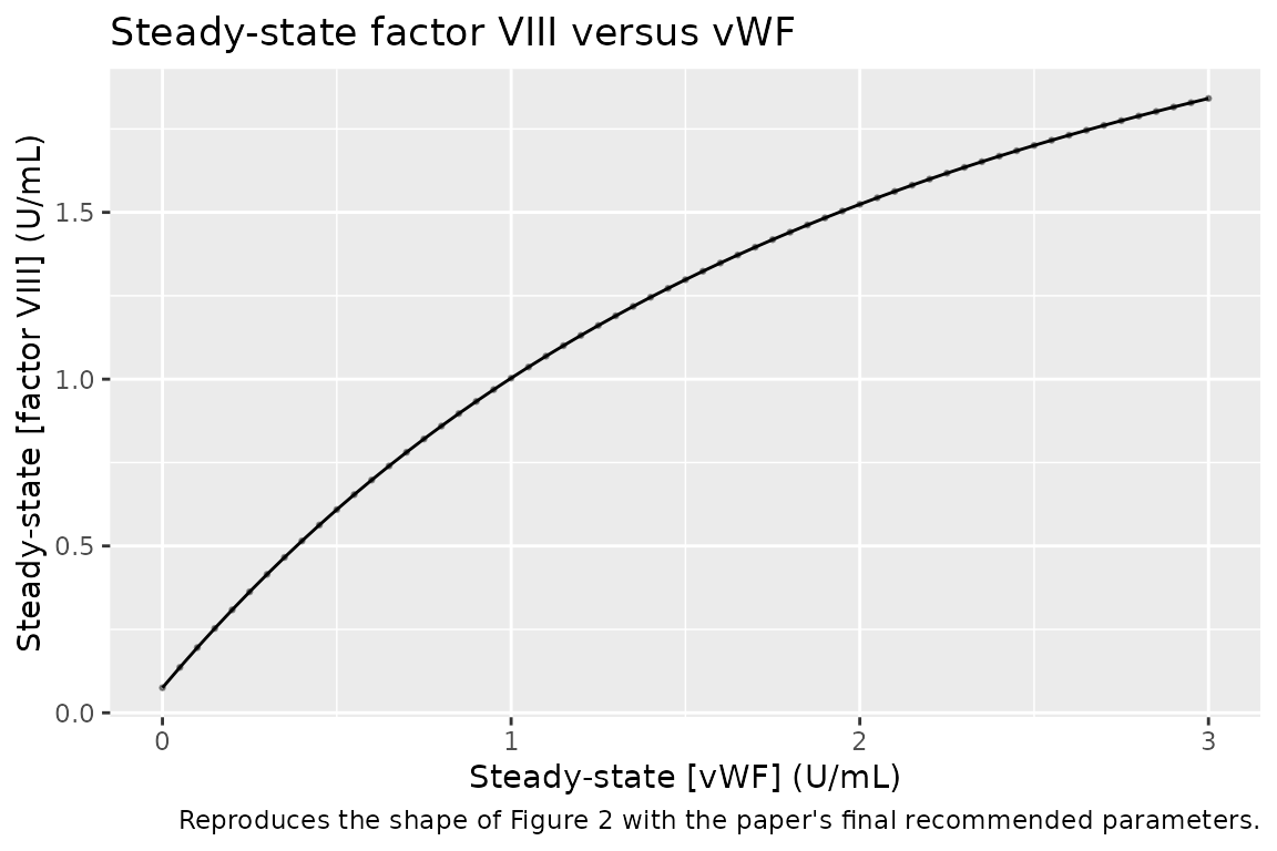

At [vWF]_ss = 0 the simulated [factor VIII]_ss is Svm/kfviii = 0.075 (type 3 vWD asymptote); at high [vWF]_ss it approaches Svm/kbviii = 3.0 U/mL (the free-form-eliminated fraction becomes negligible). The paper’s Figure 2 uses Svm/kfviii = 0.05 rather than the recommended 0.075; overriding via rxode2::ini(lsvmkfviii = log(0.05)) reproduces the family of curves at the paper’s chosen value.

Assumptions and deviations

No inter-individual variability, no residual error. The paper reports point estimates fit to mean literature data across clinical settings; no eta* or propSd parameters are declared.
Quasi-equilibrium reduction. The four ODEs of the paper are collapsed to two ODEs plus one algebraic mass-action solve, valid under the paper’s own approximation kequi ~= kd (which requires kvWF << koff, kon; the paper never reports kon and koff individually). This is a lossless reduction under the paper’s stated assumption.
Reference state / initial conditions. viii(0) = bl_viii = 1.0 U/mL and vwf(0) = bl_vwf = 1.0 U/mL are defaults for a normal healthy adult. For alternative populations, override via rxode2::ini(bl_vwf = ..., bl_viii = ...) and, where the population implies a different endogenous synthesis rate, also override lsvmkfviii (severe hemophilia: near 0; hemophilia carrier: about half normal; acute-phase / pregnancy: unchanged but bl_vwf elevated). See the scenario sections above.
Slight steady-state drift (~0.3 %). The paper’s rounded N = 4.67 gives an approximate but not exact steady state at [viii] = [vwf] = 1 U/mL; the true numerical fixed point differs by about 0.3 %. This matches the paper’s own numeric precision.
Compartment / parameter names. viii and vwf (paper-specific compartments), bl_vwf / bl_viii (baseline anchors), and lsvmkfviii (Svm/kfviii) follow the endogenous-model naming guidance (paper-native lower-case snake-case for mechanistic parameters).
Dose units. Bolus events use the state’s native units (U/mL); users with a mass dose must divide by the plasma volume (typically 40 mL/kg for adults, per Discussion p. 300) before setting amt.
PKNCA not used. This is a mechanistic endogenous physiology model; the paper does not report AUC / Cmax NCA parameters and the validation targets are steady-state, mass-balance, and figure replication (per the endogenous-validation pattern).