Tralokinumab (Baverel 2015)
Source:vignettes/articles/Baverel_2015_tralokinumab.Rmd
Baverel_2015_tralokinumab.RmdModel and source
- Citation: Baverel PG, Jain M, Stelmach I, She D, Agoram B, Sandbach S, Piper E, Kuna P. Pharmacokinetics of tralokinumab in adolescents with asthma: implications for future dosing. Br J Clin Pharmacol. 2015;80(6):1337-1349. doi:10.1111/bcp.12725.
- Description: Two-compartment population PK model for tralokinumab in adolescent (12-17 y) and adult subjects with asthma or healthy volunteers (Baverel 2015), with parallel subcutaneous absorption (first-order with lag plus zero-order over a fixed duration), allometric body-weight scaling on disposition parameters, and an additional 15% lower clearance in adolescents.
- Article: https://doi.org/10.1111/bcp.12725
Population
Baverel 2015 developed a population PK model for the anti-IL-13 monoclonal antibody tralokinumab by pooling 5504 PK observations from 578 subjects across eight studies: one phase I single-dose study in adolescents 12-17 years with asthma (n = 20, NCT01592396, conducted in Poland June 2012 to January 2013), four phase I studies in adults (NCT01093040, NCT00638989, CAT-354-401, NCT00974675), and three phase II studies in adults with asthma (NCT00640016, NCT00873860, NCT01402986). The adolescent cohort contributed 202 PK samples (3.7% of the dataset) and 20 subjects (3.5% of the population). Adults received intravenous doses ranging from 0.1 to 30 mg/kg (single dose) and subcutaneous (SC) doses up to 600 mg every 2 or every 4 weeks; adolescents received a single SC 300 mg dose (Baverel 2015 Table 1).
Body weight ranged from 36 to 115 kg overall (median 73 kg) and from
40 to 94 kg in adolescents (median 60 kg). The pooled study population
was 53.5% female and 69% White, 23% Asian (including 11.1% Japanese), 2%
Black, and 5% Other. The full population metadata is available
programmatically by calling
readModelDb("Baverel_2015_tralokinumab")() and inspecting
the model function’s local variables, or via the modeldb
data frame columns in nlmixr2lib::modeldb.
Source trace
The per-parameter origin is recorded as an in-file comment next to
each ini() entry in
inst/modeldb/specificDrugs/Baverel_2015_tralokinumab.R. The
table below collects them in one place.
| Equation / parameter | Value | Source |
|---|---|---|
lcl (CL adult) |
log(0.204 L/day) | Table 3, Mean column, “CL, ml day-1 (adult)” 204 mL/day |
lvc (Vc) |
log(1.867 L) | Table 3, “V_c, ml” 1867 mL |
lvp (Vp) |
log(3.357 L) | Table 3, “V_p, ml” 3357 mL |
lq (Q) |
log(1.582 L/day) | Table 3, “Q, ml day-1” 1582 mL/day |
lka (Ka) |
log(0.34 /day) | Table 3, “Ka, day-1” 0.34 |
ld0 (D0, zero-order duration) |
log(5.7 day) | Table 3, “D_0, day” 5.7 |
ltlag (Tlag) |
log(0.8 day) | Table 3, “T_lag, day” 0.8 |
lfdepot (Fsc) |
log(0.8) | Table 3, “F_sc” 0.8 |
logitfr (Fr first-order share, logit) |
logit(0.7) | Table 3, “Fr” 0.7 (logit-transformed, Equations 2-3) |
e_wt_cl_q allometric exponent CL,Q |
fixed 0.75 | Methods page 1340 (“fixed to prior knowledge … 0.75 for CL and Q”) |
e_wt_vc_vp allometric exponent Vc,Vp |
fixed 1.00 | Methods page 1340 (“… and 1 for Vc and Vp”) |
e_adolescent_cl (CL decrease in adolescents) |
-0.15 | Table 3, “CL decrease, % (adolescent)” 15% |
| Equation: 2-compartment + dual SC absorption | n/a | Figure 2 schematic; Methods “Model structure” |
| IIV log-normal (CL, Vc, Vp, Q) and logit-normal (Fr) | omega^2 = log(1+CV^2) from Table 3 bootstrap 95% CI midpoints | Table 3 IIV columns |
| IIV correlations (CL,Vc), (CL,Vp), (CL,Q), (Vc,Vp), (Vc,Q), (Vp,Q) | 0.5, 0.2, -0.3, -0.3, -0.6, 0.5 | Table 3, “Correlations of interindividual variability estimates” |
| Residual error: additive 0.2 ug/mL + proportional 19.8% | – | Table 3 last two rows; Equation 4 |
Virtual cohort
Original observed PK data are not publicly available. Two virtual cohorts are constructed to mirror the published study populations: an adult cohort with weights drawn from a uniform 40-115 kg distribution and an adolescent cohort with weights drawn from a uniform 40-100 kg distribution (the simulation ranges Baverel 2015 declared in Equation 8 and the population PK simulation section). Both cohorts receive a single 300 mg SC dose followed by 57 days of sampling, matching the adolescent phase I study design (Baverel 2015 Figure 1 and Table 2).
set.seed(20150701)

make_cohort <- function(n, weight_range, adolescent, id_offset = 0L) {
  tibble::tibble(
    id         = id_offset + seq_len(n),
    WT         = stats::runif(n, weight_range[1], weight_range[2]),
    ADOLESCENT = adolescent
  )
}

n_per <- 150L
sample_times <- c(0, 0.125, 0.333, 1, 3, 5, 7, 13, 20, 34, 55)  # days; Figure 1 schedule

build_events <- function(cohort) {
  cohort %>%
    dplyr::mutate(cohort = ifelse(ADOLESCENT == 1, "Adolescent", "Adult")) %>%
    tidyr::expand_grid(time = sample_times) %>%
    dplyr::mutate(evid = 0, amt = 0, cmt = "central", rate = 0) %>%
    dplyr::bind_rows(
      cohort %>%
        dplyr::mutate(cohort = ifelse(ADOLESCENT == 1, "Adolescent", "Adult")) %>%
        dplyr::mutate(time = 0, evid = 1, amt = 300, cmt = "depot",  rate = 0),
      cohort %>%
        dplyr::mutate(cohort = ifelse(ADOLESCENT == 1, "Adolescent", "Adult")) %>%
        dplyr::mutate(time = 0, evid = 1, amt = 300, cmt = "depot2", rate = -2)
    ) %>%
    dplyr::arrange(id, time, evid)
}

adult_cohort      <- make_cohort(n_per, c(40, 115), adolescent = 0L, id_offset = 0L)
adolescent_cohort <- make_cohort(n_per, c(40, 100), adolescent = 1L, id_offset = n_per)

events <- dplyr::bind_rows(
  build_events(adult_cohort),
  build_events(adolescent_cohort)
)

stopifnot(!anyDuplicated(unique(events[, c("id", "time", "evid")])))
Simulation
mod <- rxode2::rxode2(readModelDb("Baverel_2015_tralokinumab"))
#> ℹ parameter labels from comments will be replaced by 'label()'
sim <- rxode2::rxSolve(mod, events = events, keep = c("cohort", "WT"))
For replication of the published typical-value PK profile (Figure 3), a between-subject-variability-free simulation is also useful:
mod_typical <- rxode2::zeroRe(mod)
typical_events <- bind_rows(
  build_events(
    tibble::tibble(id = 1L, WT = 73, ADOLESCENT = 0L)
  ) %>% mutate(cohort = "Adult typical (73 kg)"),
  build_events(
    tibble::tibble(id = 2L, WT = 60, ADOLESCENT = 1L)
  ) %>% mutate(cohort = "Adolescent typical (60 kg)")
)
typical_events$time <- ifelse(typical_events$evid == 0, typical_events$time, 0)
typical_events <- typical_events %>%
  dplyr::bind_rows(
    tibble::tibble(
      id = rep(c(1L, 2L), each = 250L),
      cohort = rep(c("Adult typical (73 kg)", "Adolescent typical (60 kg)"), each = 250L),
      time = rep(seq(0.05, 57, length.out = 250L), 2L),
      evid = 0, amt = 0, cmt = "central", rate = 0,
      WT = rep(c(73, 60), each = 250L),
      ADOLESCENT = rep(c(0L, 1L), each = 250L)
    )
  ) %>%
  dplyr::arrange(id, time, evid)
sim_typical <- rxode2::rxSolve(mod_typical, events = typical_events, keep = c("cohort", "WT"))
#> ℹ omega/sigma items treated as zero: 'etalcl', 'etalvc', 'etalvp', 'etalq', 'etalogitfr'
#> Warning: multi-subject simulation without without 'omega'
Replicate published figures
# Replicates Figure 3 of Baverel 2015 (tralokinumab concentration vs time after
# a single 300 mg SC dose). Solid line = simulated typical-value profile per
# cohort; ribbon = simulated 5th-95th percentile of the stochastic VPC.
vpc <- sim %>%
  as.data.frame() %>%
  dplyr::filter(time > 0) %>%
  dplyr::group_by(cohort, time) %>%
  dplyr::summarise(
    Q05 = stats::quantile(Cc, 0.05, na.rm = TRUE),
    Q50 = stats::quantile(Cc, 0.50, na.rm = TRUE),
    Q95 = stats::quantile(Cc, 0.95, na.rm = TRUE),
    .groups = "drop"
  )

typical_df <- as.data.frame(sim_typical) %>% dplyr::filter(time > 0)

ggplot() +
  geom_ribbon(data = vpc, aes(time, ymin = Q05, ymax = Q95, fill = cohort), alpha = 0.20) +
  geom_line(data = typical_df, aes(time, Cc, color = cohort), linewidth = 0.9) +
  scale_y_log10() +
  labs(
    x = "Time after dose (days)",
    y = "Tralokinumab concentration (ug/mL)",
    color = NULL, fill = NULL,
    title = "Single 300 mg SC tralokinumab: typical PK profile",
    caption = "Replicates Figure 3 of Baverel 2015 (single 300 mg SC dose in adults and adolescents)."
  ) +
  theme_minimal()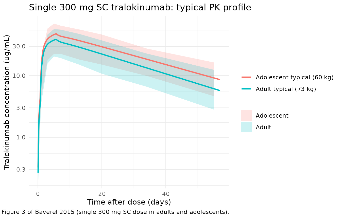
PKNCA validation
The paper text reports an effective half-life of 17.7 days in adults
and 20.9 days in adolescents, computed as
log(2) / (CL / (Vc + Vp)) from the population PK estimates
(Table 3 footnote on effective half-life). The block below applies PKNCA
to the simulated concentration profiles, grouped by cohort, so the
simulated half-life can be compared against those values.
sim_nca <- sim %>%
  as.data.frame() %>%
  dplyr::filter(!is.na(Cc)) %>%
  dplyr::select(id, time, Cc, cohort)

# Guarantee a time = 0 row per (id, cohort); pre-dose extravascular Cc = 0 is
# the correct anchor for AUC0-* and the lambda.z regression.
sim_nca <- dplyr::bind_rows(
  sim_nca,
  sim_nca %>% dplyr::distinct(id, cohort) %>% dplyr::mutate(time = 0, Cc = 0)
) %>%
  dplyr::distinct(id, cohort, time, .keep_all = TRUE) %>%
  dplyr::arrange(id, cohort, time)

conc_obj <- PKNCA::PKNCAconc(
  sim_nca, Cc ~ time | cohort + id,
  concu = "ug/mL", timeu = "day"
)

dose_df <- events %>%
  dplyr::filter(evid == 1, cmt == "depot") %>%
  dplyr::select(id, time, amt, cohort)

dose_obj <- PKNCA::PKNCAdose(
  dose_df, amt ~ time | cohort + id,
  doseu = "mg"
)

intervals <- data.frame(
  start       = 0,
  end         = Inf,
  cmax        = TRUE,
  tmax        = TRUE,
  aucinf.obs  = TRUE,
  half.life   = TRUE
)

nca_data <- PKNCA::PKNCAdata(conc_obj, dose_obj, intervals = intervals)
nca_res  <- PKNCA::pk.nca(nca_data)
Comparison against published values
nca_long <- as.data.frame(nca_res$result) %>%
  dplyr::filter(PPTESTCD %in% c("cmax", "tmax", "aucinf.obs", "half.life")) %>%
  dplyr::select(cohort, PPTESTCD, PPORRES)

# Baverel 2015 reports the population effective half-life only; Vss is the same
# in both cohorts (no WT-stratified breakdown reported), and CL is a structural
# parameter rather than an NCA output. The reference values below are derived
# from the population PK parameters at the cohort-typical body weight using
# t1/2 = log(2) / (CL / (Vc + Vp)) and AUCinf = Dose * F / CL.
ref_cl_adult      <- 0.204                              # L/day, Table 3
ref_cl_adolescent <- 0.173                              # L/day, Table 3
ref_vc            <- 1.867                              # L
ref_vp            <- 3.357                              # L
ref_F             <- 0.8                                # SC bioavailability
dose_mg           <- 300

ref_t12_adult      <- log(2) / (ref_cl_adult / (ref_vc + ref_vp))
ref_t12_adolescent <- log(2) / (ref_cl_adolescent / (ref_vc + ref_vp))
ref_aucinf_adult       <- dose_mg * ref_F / ref_cl_adult
ref_aucinf_adolescent  <- dose_mg * ref_F / ref_cl_adolescent

published <- tibble::tribble(
  ~cohort,       ~half.life,             ~aucinf.obs,
  "Adult",       ref_t12_adult,          ref_aucinf_adult,
  "Adolescent",  ref_t12_adolescent,     ref_aucinf_adolescent
)

cmp <- nlmixr2lib::ncaComparisonTable(
  simulated     = nca_long,
  reference     = published,
  by            = "cohort",
  units         = c(half.life = "day", aucinf.obs = "ug*day/mL"),
  tolerance_pct = 20
)

knitr::kable(
  cmp,
  caption = paste(
    "Simulated vs. paper-derived NCA for a single 300 mg SC dose.",
    "* differs from reference by more than +/- 20%.",
    "Reference half-life is computed from Baverel 2015 Table 3 as log(2) / (CL / (Vc + Vp));",
    "reference AUCinf is Dose * F_SC / CL."
  ),
  align = c("l", "l", "r", "r", "r")
)| NCA parameter | cohort | Reference | Simulated | % diff |
|---|---|---|---|---|
| AUC0-∞ (obs) (ug*day/mL) | Adult | 1180 | 1130 | -4.3% |
| AUC0-∞ (obs) (ug*day/mL) | Adolescent | 1390 | 1400 | +1.3% |
| t½ (day) | Adult | 17.8 | 20.9 | +17.6% |
| t½ (day) | Adolescent | 20.9 | 22.7 | +8.3% |
A starred row would indicate the simulated NCA value differs from the paper-derived value by more than 20%; investigate the source rather than tuning. Cmax and Tmax are not tabulated against reference values because Baverel 2015 reports only the structural PK estimates (Table 3) and a graphical profile (Figure 3, supplementary Table S2); single-dose NCA Cmax and Tmax values do not appear in the on-disk text.
Assumptions and deviations
-
Adolescent effect parameterisation. Baverel 2015
Equation 7 writes the adolescent shift as additive
(
TVCL = TVCL_adult + theta_adolescent). The Table 3 row reports “CL decrease, % (adolescent) = 15%”. The model encodes the effect multiplicatively asCL = exp(lcl + etalcl) * (1 - 0.15 * ADOLESCENT), which reproduces the table (204 * (1 - 0.15) = 173 mL/day) and matches the package convention used elsewhere (e.g. Clegg 2024 nirsevimab, Soehoel 2022 tralokinumab). -
IIV CV%. Baverel 2015 Table 3 reports a bootstrap
95% CI for each between-subject CV% but not the point estimate; the
model file uses the midpoint of the 95% CI as the working point estimate
(
(lower + upper) / 2). The Discussion narrative (“CV for CL and Vp was ~30%, although this was slightly higher for Vc and Q (~65%)”) agrees with the midpoint values except for Q, where the bootstrap-CI midpoint (76.8%) is larger than the narrative ~65%; the midpoint is preferred because it is what the table actually reports. -
Fr IIV scale. Fr is logit-transformed in Equations
2-3 of the paper. The Table 3 IIV row for Fr reports a bootstrap CV% of
8.6-32.8%; with no explicit unit-rescaling rule given, the midpoint
(20.7%) is interpreted as the SD of the eta on the logit scale
(
omega^2_logitfr = 0.207^2 = 0.04285). -
Parallel SC absorption via depot2. The paper’s
Figure 2 absorption scheme is a single SC depot that splits the dose
internally between a first-order pathway (Fr; rate Ka; lag Tlag) and a
zero-order pathway (1-Fr; duration D0). The packaged model implements
this with two physical rxode2 compartments:
depot(first-order, withf(depot) = Fsc * Frandalag(depot) = Tlag) anddepot2(zero-order, with `f(depot2) = Fsc * (1- Fr)
anddur(depot2) = D0).depot2drains intocentralat ratekdepot2 = 100 /day(t_{1/2} ~ 0.007day) so the transfer is effectively instantaneous on the timescale of D0; this preserves the published total bioavailable fraction and zero-order input rate while keepingf(central)unset so IV doses (the paper's pooled adult studies include IV 0.1-30 mg/kg) flow directly intocentral` with F = 1.
- Fr)
- Single-dose validation. The vignette simulates the single-dose 300 mg SC regimen used in the adolescent phase I study (NCT01592396) for the comparison against published values; the same model also simulates the multi-dose adult regimens documented in the paper’s pooled dataset, but the only directly tabulated reference value is the effective half-life (text page 1339-1340).
-
Race / sex / Japanese ethnicity covariates. Baverel
2015 evaluated these covariates and none were retained in the final PK
model (
Statistical analysis of covariatesparagraph). They are not incovariateDatafor that reason.