1,4-Butanediol bioactivation and ethanol interaction (Fung 2008) -- rat
Source:vignettes/articles/Fung_2008_butanediol_rat.Rmd
Fung_2008_butanediol_rat.RmdModel and source
- Citation: Fung HL, Tsou PS, Bulitta JB, Tran DC, Page NA, Soda D, Fung SM. Pharmacokinetics of 1,4-butanediol in rats: bioactivation to gamma-hydroxybutyric acid, interaction with ethanol, and oral bioavailability. The AAPS Journal 2008; 10(1):56-69.
- Article: doi:10.1208/s12248-007-9006-3
Population
The model was fit to plasma concentration-time data from adult male Sprague-Dawley rats (Harlan, Indianapolis, IN) of about 300 g body weight studied at the University at Buffalo. Thirteen treatment groups of 3-4 rats each (Table I of the source paper) covered:
- monotherapy IV dosing of BD (1.58 or 6.34 mmol/kg), GHB (1.58, 1.79, or 6.34 mmol/kg), and ETOH (6.34 or 12.7 mmol/kg);
- pairwise IV co-administration of BD + ETOH and of GHB + ETOH; and
- oral BD dosing by gastric gavage at 1.58 or 6.34 mmol/kg.
Each IV dose was a 5-min constant-rate infusion via femoral cannula; blood samples were taken from the jugular vein and assayed for BD and GHB by LCMS (LOQ 60 uM) and for ETOH by GC-FID. The semialdehyde intermediate (ALD) was not measured. The mixed-effects fit used NONMEM VI with the ADVAN9 stiff-system solver and the FOCE interaction option.
The same demographic and dosing summary is available programmatically
via the model’s population metadata
(readModelDb("Fung_2008_butanediol_rat")$population).
Source trace
Per-parameter origin is recorded as an in-file comment next to each
ini() entry in
inst/modeldb/specificDrugs/Fung_2008_butanediol_rat.R. The
table below collects the source locations in one place for review.
| Equation / parameter | Value | Source location |
|---|---|---|
| ODE system (BD, ALD, GHB, ETOH) | n/a | Eqs. 1-8 + Fig. 1 |
| BD Vmax (calculated) | 0.0362 mmol/min | Table II BD column (footnote a) |
| BD Km | 1.56 mmol/L | Table II BD column |
| BD Vc | 0.248 L (CV 11%) | Table II BD column |
| BD k12, k21 | 0.00231, 0.0150 1/min | Table II BD column |
| ALD Vmax (estimated) | 0.0168 mmol/min | Table II ALD column |
| ALD Km | 0.446 mmol/L | Table II ALD column |
| ALD Vc | 0.0476 L (constrained Vss_ALD = Vss_BD) | Table II ALD column (footnote c) |
| ALD k12, k21 | 0.0526, 0.0105 1/min | Table II ALD column |
| GHB linear CL | 0.00046 L/min | Table II GHB column |
| GHB Vmax (calculated) | 0.00361 mmol/min | Table II GHB column (footnote a) |
| GHB Km | 0.0906 mmol/L (CV 35%) | Table II GHB column |
| GHB Vc | 0.010 L (FIXED, rat plasma volume) | Table II GHB column (footnote b) |
| GHB k12, k21 | 0.551, 0.0554 1/min | Table II GHB column |
| ETOH Vmax (calculated) | 0.0410 mmol/min (CV 1.9% on CLic) | Table II ETOH column (footnote a) |
| ETOH Km | 0.746 mmol/L (CV 14%) | Table II ETOH column |
| ETOH Vc | 0.205 L (CV 20%) | Table II ETOH column |
| ETOH k12, k21 | 0.0338, 0.0589 1/min | Table II ETOH column |
| Ki BD inhibiting ALD | 3.67 mmol/L (CV 46%) | Table II inhibition constants |
| Ki BD inhibiting GHB | 3.56 mmol/L (CV 69%) | Table II inhibition constants |
| Ki BD inhibiting ETOH | 2.24 mmol/L (CV 37%) | Table II inhibition constants |
| Ki GHB inhibiting BD | 15.2 mmol/L (CV 25%) | Table II inhibition constants |
| Ki ETOH inhibiting BD | 0.615 mmol/L | Table II inhibition constants |
| Oral half-life of absorption (ka) | 0.98 min (-> ka = ln(2)/0.98) | Results “BD Oral Bioavailability” |
| Oral lag time (tlag) | 7.5 min (CV 10%) | Results “BD Oral Bioavailability” |
| Total oral F (BD + ALD) | 0.93 | Results “BD Oral Bioavailability” |
| Oral fr_BD (low dose default) | 0.30 at 1.58 mmol/kg | Results “BD Oral Bioavailability” |
| Oral fr_BD (high dose) | 0.55 at 6.34 mmol/kg | Results “BD Oral Bioavailability” |
| Residual error BD | prop 17.5%, add 0.0030 mmol/L | Table II BD |
| Residual error GHB | prop 12.8%, add 0.0186 mmol/L | Table II GHB |
| Residual error ETOH | prop 2.32%, add 0.233 mmol/L | Table II ETOH |
Loading the model
mod <- readModelDb("Fung_2008_butanediol_rat")
mod_typical <- rxode2::zeroRe(mod)
#> ℹ parameter labels from comments will be replaced by 'label()'
Helper to build an event table. The IV doses use a 5-min
constant-rate infusion matching the source paper’s experimental design;
the oral BD dose enters the depot compartment and is split
between systemic BD and systemic ALD via fr_bd. Doses are
in mmol (the model’s molar units); for a 300 g rat at 6.34 mmol/kg the
dose is 6.34 * 0.3 = 1.902 mmol per rat.
RAT_WT_KG <- 0.30
INF_MIN   <- 5

# Build a single-rat event table with one IV or PO dose and dense
# observation rows on the three measured analytes (BD `Cc`, GHB
# `Cc_ghb`, ETOH `Cc_etoh`). When `dose_bd_mmolkg`, `dose_ghb_mmolkg`,
# or `dose_etoh_mmolkg` is positive that compound is dosed; multiple
# can be non-zero for co-administration cohorts.
make_events <- function(dose_bd_mmolkg = 0, dose_ghb_mmolkg = 0,
                        dose_etoh_mmolkg = 0, route_bd = c("iv", "po"),
                        tmax = 300, dt = 5, id_offset = 0L) {
  route_bd <- match.arg(route_bd)
  id <- id_offset + 1L

  add_inf <- function(amt_mmol, cmt) {
    if (amt_mmol <= 0) return(NULL)
    data.frame(
      id   = id,
      time = 0,
      evid = 1,
      amt  = amt_mmol,
      rate = amt_mmol / INF_MIN,
      cmt  = cmt
    )
  }
  add_bolus <- function(amt_mmol, cmt) {
    if (amt_mmol <= 0) return(NULL)
    data.frame(
      id   = id, time = 0, evid = 1, amt = amt_mmol,
      rate = 0, cmt = cmt
    )
  }

  dose_bd_mmol   <- dose_bd_mmolkg   * RAT_WT_KG
  dose_ghb_mmol  <- dose_ghb_mmolkg  * RAT_WT_KG
  dose_etoh_mmol <- dose_etoh_mmolkg * RAT_WT_KG

  bd_dose <- if (route_bd == "iv") {
    add_inf(dose_bd_mmol, "central")
  } else {
    add_bolus(dose_bd_mmol, "depot")
  }

  doses <- dplyr::bind_rows(
    bd_dose,
    add_inf(dose_ghb_mmol,  "central_ghb"),
    add_inf(dose_etoh_mmol, "central_etoh")
  )

  obs <- tidyr::expand_grid(
    id   = id,
    time = seq(0, tmax, by = dt),
    cmt  = c("Cc", "Cc_ghb", "Cc_etoh")
  ) %>%
    dplyr::mutate(evid = 0, amt = 0, rate = 0) %>%
    dplyr::select(id, time, evid, amt, rate, cmt)

  dplyr::bind_rows(doses, obs)
}
Replicating Figure 4: BD IV dosed alone, at low and high doses
Figure 4 of the source paper shows the median model predictions for plasma BD (panels a-b) and the metabolically generated GHB (panels e-f) after IV BD alone at 1.58 and 6.34 mmol/kg. Panels c-d show the unmonitored ALD intermediate. Below is the typical-value reproduction from the packaged model.
ev_bd_low  <- make_events(dose_bd_mmolkg = 1.58)
ev_bd_high <- make_events(dose_bd_mmolkg = 6.34)

sim_bd_low  <- as.data.frame(rxSolve(mod_typical, ev_bd_low))
#> ℹ omega/sigma items treated as zero: 'etalvmax', 'etalvc', 'etalkm_ghb', 'etalvc_ghb', 'etalvmax_etoh', 'etalkm_etoh', 'etalvc_etoh', 'etalki_bd_ald', 'etalki_bd_ghb', 'etalki_bd_etoh', 'etalki_ghb_bd', 'etaltlag'
sim_bd_high <- as.data.frame(rxSolve(mod_typical, ev_bd_high))
#> ℹ omega/sigma items treated as zero: 'etalvmax', 'etalvc', 'etalkm_ghb', 'etalvc_ghb', 'etalvmax_etoh', 'etalkm_etoh', 'etalvc_etoh', 'etalki_bd_ald', 'etalki_bd_ghb', 'etalki_bd_etoh', 'etalki_ghb_bd', 'etaltlag'

bd_iv_long <- dplyr::bind_rows(
  sim_bd_low  %>% dplyr::mutate(dose = "1.58 mmol/kg"),
  sim_bd_high %>% dplyr::mutate(dose = "6.34 mmol/kg")
) %>%
  tidyr::pivot_longer(c(Cc, Cc_ald, Cc_ghb),
                      names_to = "analyte", values_to = "conc") %>%
  dplyr::mutate(analyte = factor(
    analyte, levels = c("Cc", "Cc_ald", "Cc_ghb"),
    labels = c("BD", "ALD (unmeasured)", "GHB (metabolite)")
  ))

ggplot(bd_iv_long, aes(time, pmax(conc, 1e-3), colour = dose)) +
  geom_line(linewidth = 0.7) +
  facet_wrap(~ analyte) +
  scale_y_log10() +
  labs(x = "Time (min)", y = "Plasma concentration (mmol/L)",
       colour = "BD IV dose",
       title = "Figure 4 replicate -- typical-value profiles for BD IV alone",
       caption = "Replicates Figure 4 of Fung 2008 (median predictions).")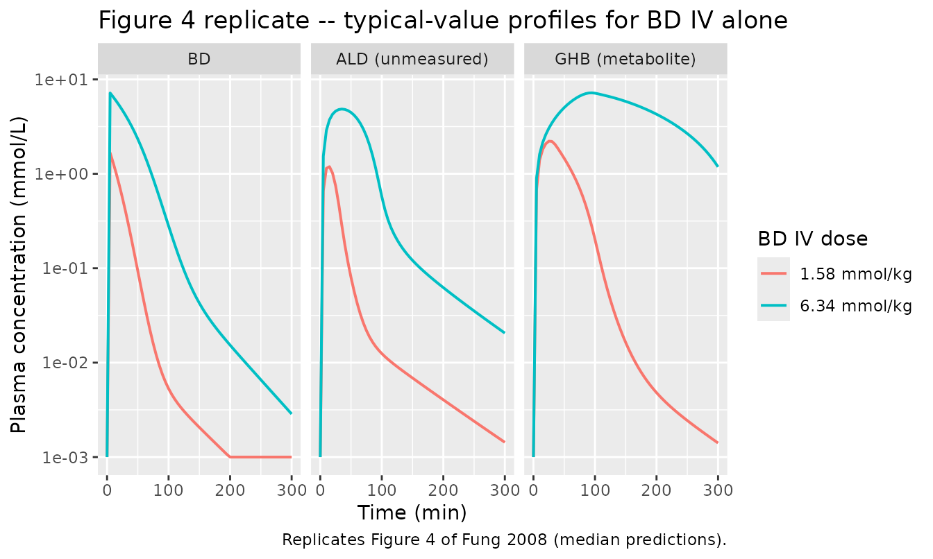
Replicating Figure 2: ETOH IV dosed alone
ev_etoh_low  <- make_events(dose_etoh_mmolkg = 6.34)
ev_etoh_high <- make_events(dose_etoh_mmolkg = 12.7)

sim_etoh <- dplyr::bind_rows(
  as.data.frame(rxSolve(mod_typical, ev_etoh_low))  %>%
    dplyr::mutate(dose = "6.34 mmol/kg"),
  as.data.frame(rxSolve(mod_typical, ev_etoh_high)) %>%
    dplyr::mutate(dose = "12.7 mmol/kg")
)
#> ℹ omega/sigma items treated as zero: 'etalvmax', 'etalvc', 'etalkm_ghb', 'etalvc_ghb', 'etalvmax_etoh', 'etalkm_etoh', 'etalvc_etoh', 'etalki_bd_ald', 'etalki_bd_ghb', 'etalki_bd_etoh', 'etalki_ghb_bd', 'etaltlag'
#> ℹ omega/sigma items treated as zero: 'etalvmax', 'etalvc', 'etalkm_ghb', 'etalvc_ghb', 'etalvmax_etoh', 'etalkm_etoh', 'etalvc_etoh', 'etalki_bd_ald', 'etalki_bd_ghb', 'etalki_bd_etoh', 'etalki_ghb_bd', 'etaltlag'

ggplot(sim_etoh, aes(time, pmax(Cc_etoh, 1e-3), colour = dose)) +
  geom_line(linewidth = 0.7) +
  scale_y_log10() +
  labs(x = "Time (min)", y = "Plasma ETOH (mmol/L)",
       colour = "ETOH IV dose",
       title = "Figure 2 replicate -- typical-value ETOH profiles",
       caption = "Replicates Figure 2 of Fung 2008.")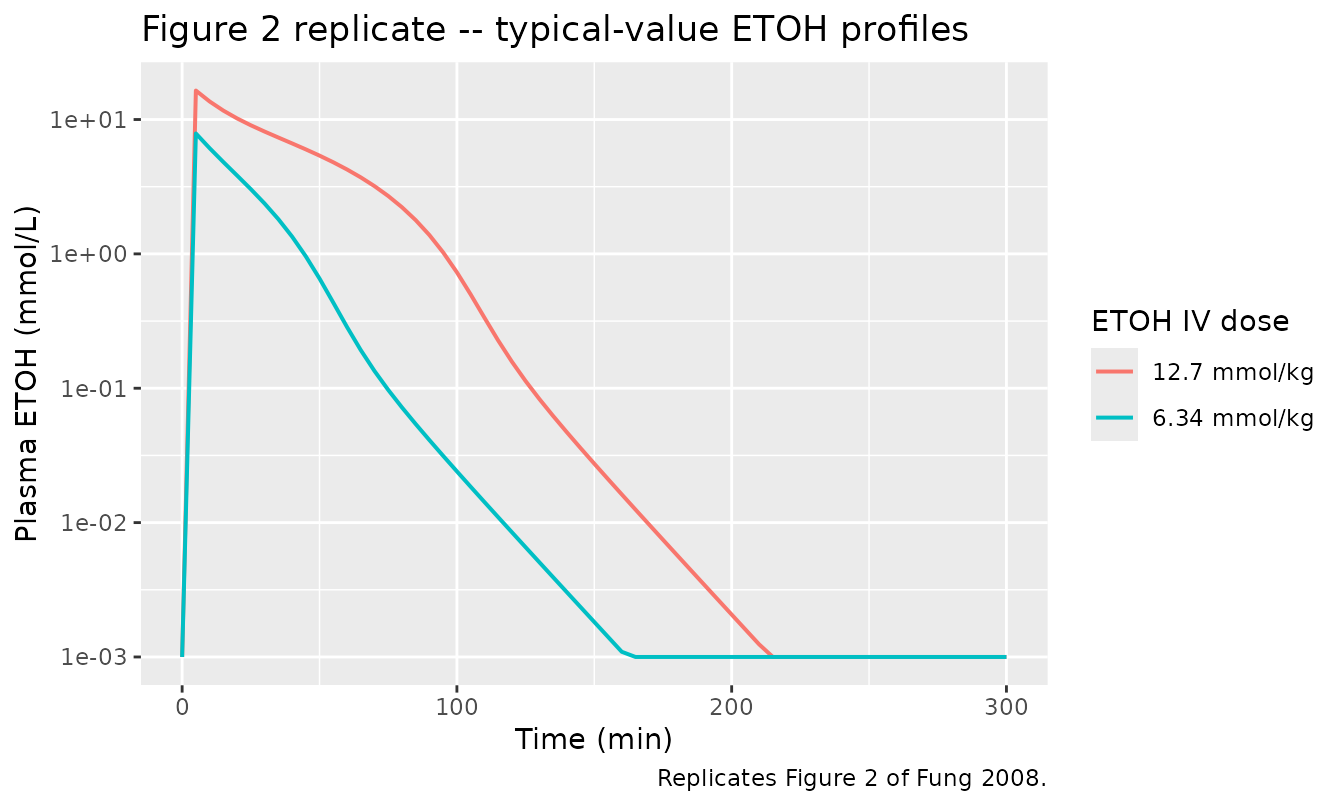
Replicating Figure 5: BD + ETOH co-administration
Figure 5 of the source paper shows the BD + ETOH co-administration
cohorts at three dose pairs. The mutual inhibition of BD elimination by
ETOH (Ki_ETOH/BD = 0.615 mmol/L) and of ETOH elimination by
BD (Ki_BD/ETOH = 2.24 mmol/L) prolongs both compounds’
exposure.
ev_co_1 <- make_events(dose_bd_mmolkg = 1.58, dose_etoh_mmolkg = 6.34)
ev_co_2 <- make_events(dose_bd_mmolkg = 1.58, dose_etoh_mmolkg = 12.7)
ev_co_3 <- make_events(dose_bd_mmolkg = 6.34, dose_etoh_mmolkg = 6.34)

sim_co <- dplyr::bind_rows(
  as.data.frame(rxSolve(mod_typical, ev_co_1)) %>%
    dplyr::mutate(panel = "BD 1.58 + ETOH 6.34"),
  as.data.frame(rxSolve(mod_typical, ev_co_2)) %>%
    dplyr::mutate(panel = "BD 1.58 + ETOH 12.7"),
  as.data.frame(rxSolve(mod_typical, ev_co_3)) %>%
    dplyr::mutate(panel = "BD 6.34 + ETOH 6.34")
) %>%
  tidyr::pivot_longer(c(Cc, Cc_etoh, Cc_ghb),
                      names_to = "analyte", values_to = "conc") %>%
  dplyr::mutate(analyte = factor(
    analyte, levels = c("Cc_etoh", "Cc", "Cc_ghb"),
    labels = c("ETOH", "BD", "GHB (metabolite)")
  ))
#> ℹ omega/sigma items treated as zero: 'etalvmax', 'etalvc', 'etalkm_ghb', 'etalvc_ghb', 'etalvmax_etoh', 'etalkm_etoh', 'etalvc_etoh', 'etalki_bd_ald', 'etalki_bd_ghb', 'etalki_bd_etoh', 'etalki_ghb_bd', 'etaltlag'
#> ℹ omega/sigma items treated as zero: 'etalvmax', 'etalvc', 'etalkm_ghb', 'etalvc_ghb', 'etalvmax_etoh', 'etalkm_etoh', 'etalvc_etoh', 'etalki_bd_ald', 'etalki_bd_ghb', 'etalki_bd_etoh', 'etalki_ghb_bd', 'etaltlag'
#> ℹ omega/sigma items treated as zero: 'etalvmax', 'etalvc', 'etalkm_ghb', 'etalvc_ghb', 'etalvmax_etoh', 'etalkm_etoh', 'etalvc_etoh', 'etalki_bd_ald', 'etalki_bd_ghb', 'etalki_bd_etoh', 'etalki_ghb_bd', 'etaltlag'

ggplot(sim_co, aes(time, pmax(conc, 1e-3), colour = analyte)) +
  geom_line(linewidth = 0.7) +
  facet_wrap(~ panel) +
  scale_y_log10() +
  labs(x = "Time (min)", y = "Plasma concentration (mmol/L)",
       colour = "Analyte",
       title = "Figure 5 replicate -- BD + ETOH IV co-administration",
       caption = "Replicates Figure 5 of Fung 2008 (typical-value).")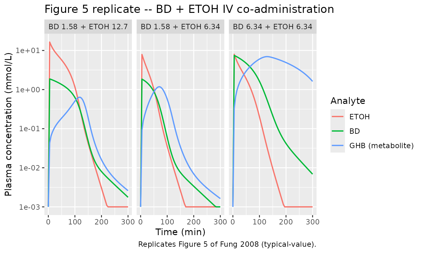
Replicating Figure 7: oral BD dosing
Figure 7 of the source paper shows individual BD, ALD, and GHB
concentrations after oral BD dosing at 1.58 mmol/kg (panel a) and 6.34
mmol/kg (panel b). The model defaults to the low-dose
fr_bd = 0.30 (i.e. 30% of the absorbed dose enters systemic
circulation as BD, 70% as ALD). For the high-dose profile we override
the loaded model’s fr_bd via the logitfr_bd
parameter so that fr_bd = 0.55.
ev_po_low_default  <- make_events(dose_bd_mmolkg = 1.58, route_bd = "po", tmax = 240)
ev_po_high_default <- make_events(dose_bd_mmolkg = 6.34, route_bd = "po", tmax = 240)

# Build a high-dose-fr variant by overriding the population fixed-effect.
qlogis55 <- qlogis(0.55)

sim_po_low  <- as.data.frame(rxSolve(mod_typical, ev_po_low_default))
#> ℹ omega/sigma items treated as zero: 'etalvmax', 'etalvc', 'etalkm_ghb', 'etalvc_ghb', 'etalvmax_etoh', 'etalkm_etoh', 'etalvc_etoh', 'etalki_bd_ald', 'etalki_bd_ghb', 'etalki_bd_etoh', 'etalki_ghb_bd', 'etaltlag'
sim_po_high <- as.data.frame(rxSolve(mod_typical, ev_po_high_default,
                                     params = c(logitfr_bd = qlogis55)))
#> ℹ omega/sigma items treated as zero: 'etalvmax', 'etalvc', 'etalkm_ghb', 'etalvc_ghb', 'etalvmax_etoh', 'etalkm_etoh', 'etalvc_etoh', 'etalki_bd_ald', 'etalki_bd_ghb', 'etalki_bd_etoh', 'etalki_ghb_bd', 'etaltlag'

po_long <- dplyr::bind_rows(
  sim_po_low  %>% dplyr::mutate(dose = "1.58 mmol/kg (fr_bd = 0.30)"),
  sim_po_high %>% dplyr::mutate(dose = "6.34 mmol/kg (fr_bd = 0.55)")
) %>%
  tidyr::pivot_longer(c(Cc, Cc_ald, Cc_ghb),
                      names_to = "analyte", values_to = "conc") %>%
  dplyr::mutate(analyte = factor(
    analyte, levels = c("Cc", "Cc_ald", "Cc_ghb"),
    labels = c("BD", "ALD (unmeasured)", "GHB (metabolite)")
  ))

ggplot(po_long, aes(time, pmax(conc, 1e-3), colour = dose)) +
  geom_line(linewidth = 0.7) +
  facet_wrap(~ analyte) +
  scale_y_log10() +
  labs(x = "Time (min)", y = "Plasma concentration (mmol/L)",
       colour = "Oral BD dose",
       title = "Figure 7 replicate -- typical-value profiles for BD PO",
       caption = "Replicates Figure 7 of Fung 2008 (typical-value).")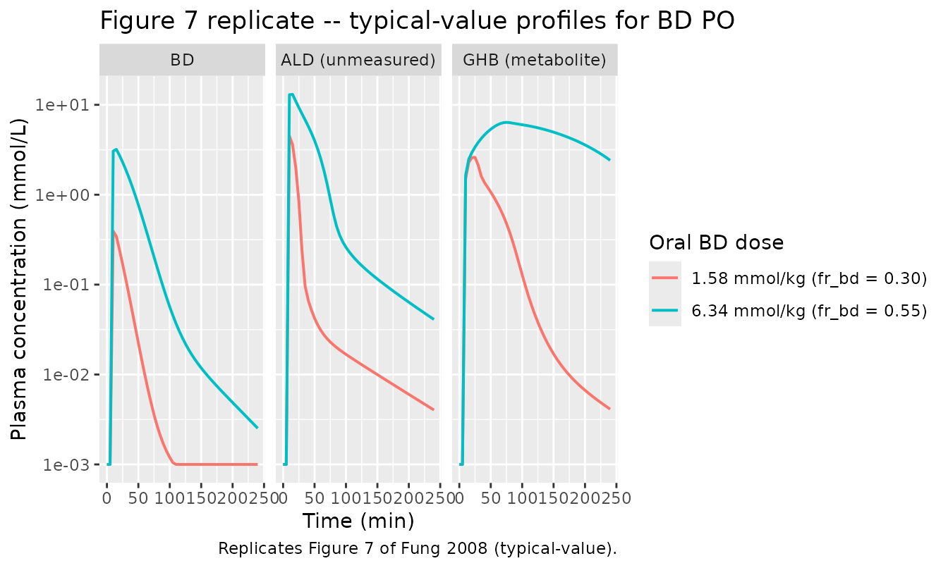
PKNCA validation: BD IV alone
Because the source paper reports analyte AUC values for the oral BD arms but not for the IV arms in a directly comparable form, the PKNCA block below summarises the simulated IV BD typical-value exposure (BD parent + the GHB metabolite generated from BD) at the two studied doses. The Cmax and AUC ratios across the 4-fold dose increase are the quantitative diagnostic: a linear-PK system would show a 4-fold increase in both, whereas the saturable elimination here yields a larger-than-proportional AUC increase that matches the Results section narrative (“nonlinear PK were also operative”).
nca_dose_table <- function(sim, dose_label) {
  sim_unique <- sim %>%
    dplyr::distinct(time, .keep_all = TRUE)

  conc_obj_bd <- PKNCAconc(sim_unique %>%
                             dplyr::transmute(id = 1L, time, Cc, treatment = dose_label),
                           Cc ~ time | treatment + id,
                           concu = "mmol/L", timeu = "min")
  conc_obj_ghb <- PKNCAconc(sim_unique %>%
                              dplyr::transmute(id = 1L, time, Cc = Cc_ghb,
                                               treatment = dose_label),
                            Cc ~ time | treatment + id,
                            concu = "mmol/L", timeu = "min")

  dose_amt <- 1.58 * (dose_label == "1.58 mmol/kg") + 6.34 * (dose_label == "6.34 mmol/kg")
  dose_df  <- data.frame(id = 1L, time = 0,
                         amt = dose_amt * RAT_WT_KG,
                         treatment = dose_label)
  dose_obj <- PKNCAdose(dose_df, amt ~ time | treatment + id, doseu = "mmol")

  intervals <- data.frame(start = 0, end = 300,
                          cmax = TRUE, tmax = TRUE,
                          auclast = TRUE, clast.obs = TRUE)

  res_bd <- pk.nca(PKNCAdata(conc_obj_bd, dose_obj, intervals = intervals))
  res_gh <- pk.nca(PKNCAdata(conc_obj_ghb, dose_obj, intervals = intervals))

  list(BD = as.data.frame(res_bd$result), GHB = as.data.frame(res_gh$result))
}

nca_low  <- nca_dose_table(sim_bd_low,  "1.58 mmol/kg")
nca_high <- nca_dose_table(sim_bd_high, "6.34 mmol/kg")

extract_row <- function(nca, label, analyte) {
  out <- nca[[analyte]] %>%
    dplyr::filter(PPTESTCD %in% c("cmax", "tmax", "auclast")) %>%
    dplyr::select(PPTESTCD, PPORRES) %>%
    tidyr::pivot_wider(names_from = PPTESTCD, values_from = PPORRES)
  dplyr::mutate(out, dose = label, analyte = analyte, .before = 1)
}

nca_tbl <- dplyr::bind_rows(
  extract_row(nca_low,  "1.58 mmol/kg", "BD"),
  extract_row(nca_low,  "1.58 mmol/kg", "GHB"),
  extract_row(nca_high, "6.34 mmol/kg", "BD"),
  extract_row(nca_high, "6.34 mmol/kg", "GHB")
)
knitr::kable(nca_tbl, digits = 3,
caption = "Typical-value NCA after IV BD (no IIV). cmax in mmol/L, auclast in mmol/L*min.")| dose | analyte | auclast | cmax | tmax |
|---|---|---|---|---|
| 1.58 mmol/kg | BD | 33.143 | 1.665 | 5 |
| 1.58 mmol/kg | GHB | 124.263 | 2.216 | 25 |
| 6.34 mmol/kg | BD | 281.432 | 7.173 | 5 |
| 6.34 mmol/kg | GHB | 1316.352 | 7.199 | 95 |
PKNCA comparison against published oral BD AUC
The source paper reports non-compartmental AUC0-inf for oral BD: mean +/- SD 8.72 +/- 5.33 mMmin at 1.58 mmol/kg and 117 +/- 82 mMmin at 6.34 mmol/kg (Results “BD Oral Bioavailability”). The 13-fold increase across a 4-fold dose increase confirms the saturable disposition. The typical-value AUC computed from the packaged model should fall near the reported means; deviation is expected because the published mean folds in inter-animal variability the typical-value path does not simulate.
nca_po_table <- function(sim, dose_label) {
  sim_unique <- sim %>% dplyr::distinct(time, .keep_all = TRUE)
  conc <- PKNCAconc(sim_unique %>%
                      dplyr::transmute(id = 1L, time, Cc, treatment = dose_label),
                    Cc ~ time | treatment + id,
                    concu = "mmol/L", timeu = "min")
  dose_amt <- 1.58 * (dose_label == "1.58 mmol/kg") + 6.34 * (dose_label == "6.34 mmol/kg")
  dose_df  <- data.frame(id = 1L, time = 0,
                         amt = dose_amt * RAT_WT_KG, treatment = dose_label)
  dose_obj <- PKNCAdose(dose_df, amt ~ time | treatment + id, doseu = "mmol")
  intervals <- data.frame(start = 0, end = 240,
                          cmax = TRUE, tmax = TRUE, auclast = TRUE)
  res <- pk.nca(PKNCAdata(conc, dose_obj, intervals = intervals))
  as.data.frame(res$result) %>%
    dplyr::filter(PPTESTCD %in% c("cmax", "tmax", "auclast")) %>%
    dplyr::select(PPTESTCD, PPORRES) %>%
    tidyr::pivot_wider(names_from = PPTESTCD, values_from = PPORRES) %>%
    dplyr::mutate(dose = dose_label, .before = 1)
}

po_nca <- dplyr::bind_rows(
  nca_po_table(sim_po_low,  "1.58 mmol/kg"),
  nca_po_table(sim_po_high, "6.34 mmol/kg")
) %>%
  dplyr::mutate(published_AUC0_inf_mean = c(8.72, 117),
                published_AUC0_inf_sd   = c(5.33, 82))

knitr::kable(po_nca, digits = 3,
caption = "Oral BD: simulated (auclast, mmol/L*min) vs published AUC0-inf (mean +/- SD).")| dose | auclast | cmax | tmax | published_AUC0_inf_mean | published_AUC0_inf_sd |
|---|---|---|---|---|---|
| 1.58 mmol/kg | 7.493 | 0.392 | 10 | 8.72 | 5.33 |
| 6.34 mmol/kg | 101.921 | 3.196 | 15 | 117.00 | 82.00 |
Assumptions and deviations
-
Drug field correction. The dispatcher metadata
field
drug = "The AAPS Journal"was a parser artefact (the journal name was mis-extracted as the drug name). The paper is unambiguously about 1,4-butanediol (BD) with the metabolite GHB and the interactant ethanol; the model filename, function name, vignette basename, and description were silently corrected to usebutanediolper the skill’s Phase 1 step 2 (paper-not-ambiguous arm). -
Dose-dependent fractional pre-systemic conversion.
The fraction of the absorbed oral BD dose entering systemic circulation
as BD versus ALD was estimated separately for each dose level in the
source paper (30% / 70% at 1.58 mmol/kg; 55% / 45% at 6.34 mmol/kg). The
encoded model uses the low-dose value (30%) as the default; to simulate
the high-dose split, override
logitfr_bd = qlogis(0.55)inrxSolve(..., params = ...)as shown in the Figure 7 chunk above. The packaged model does not encode a mechanistic dose-saturable pre-systemic metabolism: the source paper reports only the two empirical fractions and notes that “pre-systemic metabolism to ALD might have become more saturated at the higher dose, although further studies are required to confirm this speculation” (Discussion). -
CLic vs Vmax parameterisation. For BD, GHB, and
ETOH the source’s Table II reports
Vmaxas the calculated quantity (Vmax = CLic * Km) andCLicas the estimated parameter; for ALD the estimated parameter isVmaxdirectly. The encoded model useslvmaxandlkmas the primaryini()parameters throughout for naming uniformity. BecauseKmfor BD and ETOH has no IIV in the source, attaching theCLicIIV toVmaxis mathematically equivalent under a constant-Km typical scaling (Vmax = CLic * KmwithKmconstant). The model file’s per-parameter source-trace comments document the back-translation. -
Vss_ALD constraint. Vss_ALD was assumed equal to
Vss_BD in the source paper (Table II footnote c) because ALD
concentrations were not measured. The encoded
V_ALD,k12_ALD, andk21_ALDvalues satisfy this constraint exactly:V_ALD * (1 + k12_ALD/k21_ALD) = 0.0476 * (1 + 0.0526 / 0.0105) = 0.286 L, matching the BD Vss reported in Table II. -
GHB V central fixed. V_GHB was fixed to the average
rat plasma volume of 0.010 L (Table II footnote b). The reported IIV on
V_GHB (16%) is included as an
etalvc_ghbterm even though the typical value is structurally fixed; downstream simulation paths that zero-out random effects (e.g.rxode2::zeroRe(mod)) recover the exact fixed value. - No covariates. Body weight, age, and sex were not modelled as covariates in the source paper – the cohort was a uniform 300 g adult male Sprague-Dawley population, so no covariate scaling is required for in-cohort simulation. Allometric or species-scaling extrapolations for cross-species predictions are out of scope for this packaged model.