Tobramycin (Downes 2022)
Source:vignettes/articles/Downes_2022_tobramycin.Rmd
Downes_2022_tobramycin.RmdModel and source
- Citation: Downes KJ, Grim A, Shanley L, Rubenstein RC, Zuppa AF, Gastonguay MR. A Pharmacokinetic Analysis of Tobramycin in Patients Less than Five Years of Age with Cystic Fibrosis: Assessment of Target Attainment with Extended-Interval Dosing through Simulation. Antimicrob Agents Chemother. 2022;66(5):e02377-21. doi:10.1128/aac.02377-21
- Description: Two-compartment IV population PK model for tobramycin in hospitalized children less than 5 years of age with cystic fibrosis treated for a pulmonary exacerbation (Downes 2022). Clearance and intercompartmental clearance scale allometrically with body weight (exponent 0.75, reference 70 kg) while central and peripheral volumes scale linearly with body weight (exponent 1, reference 70 kg). Clearance additionally carries a power effect of age (exponent 0.136, reference 2.7 years), a power effect of bedside-Schwartz estimated GFR (exponent 0.246, reference 128 mL/min/1.73 m^2), and a 29.2% reduction with concomitant vancomycin. Between-subject variability is a full block on clearance and central volume; residual variability is proportional.
- Article: https://doi.org/10.1128/aac.02377-21
Downes 2022 is a retrospective population PK analysis of intravenous tobramycin in hospitalized children under 5 years of age with cystic fibrosis treated for a pulmonary exacerbation. The clinical question is whether the extended-interval (once-daily) dosing that the Cystic Fibrosis Foundation recommends for patients 5 years and older can be used empirically in younger children, for whom data were lacking. The cohort itself never received extended-interval dosing: it was treated on the institution’s every-8-hour schedule, and the once-daily regimens are explored entirely by Monte Carlo simulation from the fitted model.
That structure is what makes this a good validation target. The paper’s Table 3 reports, for each of six once-daily dose levels, the percentage of simulated patients meeting five prespecified therapeutic targets, and its footnote states exactly how each target was evaluated. Those definitions are reproduced below and used as the primary validation gate.
Population
The analysis pooled 111 tobramycin courses in 58 patients treated at the Children’s Hospital of Philadelphia between March 2011 and September 2018 (Downes 2022 Table 1). Median age at the start of a first course was 2.2 years (IQR 0.8-3.8), median weight 11.2 kg (IQR 8.2-14.7), and median bedside-Schwartz eGFR 126 mL/min/1.73 m^2 (IQR 110-149); 43% were female. Renal impairment (eGFR < 60 mL/min/1.73 m^2) was an exclusion criterion and only 3 of 58 first courses (5.2%) had an eGFR below 90, so the cohort is essentially normal-to-supranormal in renal function.
The formulary starting dose for this age group was 3.3 mg/kg every 8 hours as a 30-minute infusion, and the observed first-course median was 3.2 mg/kg/dose (IQR 3.1-3.3). Only concentrations drawn within the first 48 hours of a course were analysed. Of 224 usable serum concentrations, 53 (23.7%) were below the 0.6 mg/L limit of quantification and were handled by the Beal M3 likelihood method.
Because sampling was routine therapeutic-drug-monitoring peaks and troughs, the distributional parameters were not identifiable from these data alone. Downes 2022 digitized the individual profiles of six richly sampled adult cystic fibrosis patients from an earlier publication, fit them to obtain prior distributions, and estimated the pediatric model by MAP-Bayesian penalized likelihood with informative priors on Q and V2. Between-subject variability on Q and V2 was estimated poorly and was fixed to zero in the final model.
The same information is available programmatically via the model’s
population metadata
(readModelDb("Downes_2022_tobramycin")()$population).
Source trace
| Equation / parameter | Value | Source location |
|---|---|---|
lcl (theta CL) |
6.10 L/hr/70 kg (%RSE 3.89) | Table 2, row “u CL (L/hr/70 kg)” |
lvc (theta V1) |
21.6 L/70 kg (%RSE 7.41) | Table 2, row “u V1 (L/70 kg)” |
lq (theta Q) |
4.73 L/hr/70 kg (%RSE 6.24) | Table 2, row “u Q (L/hr/70 kg)” |
lvp (theta V2) |
6.69 L/70 kg (%RSE 7.55) | Table 2, row “u V2 (L/70 kg)” |
e_wt_cl_q |
0.75 (fixed) | Results “Model development”; Table 2 footnote
[WT/70]^0.75
|
e_wt_vc_vp |
1 (fixed) | Results “Model development”; Table 2 footnote
(WT/70)
|
e_age_cl (theta AGE) |
0.136 (%RSE 12.1) | Table 2, row “u AGE” |
e_crcl_cl (theta GFR) |
0.246 (%RSE 32.4) | Table 2, row “u GFR” |
e_conmed_vancomycin_cl (theta VAN) |
0.708 (%RSE 19.1) | Table 2, row “u VAN” |
| Reference weight 70 kg | Results “Model development”; Table 2 footnote | |
| Reference age 2.7 years | Table 2 footnote, (AGE/2.7)
|
|
| Reference eGFR 128 mL/min/1.73 m^2 | Table 2 footnote, (GFR/128)
|
|
etalcl variance |
0.0296 (17.2% CV, %RSE 17.8) | Table 2, row “v 1,1-CL” |
etalcl:etalvc covariance |
0.0325 (r = 0.751, %RSE 32.3) | Table 2, row “v 1,2-CL:V1” + footnote b |
etalvc variance |
0.0633 (25.2% CV, %RSE 28.9) | Table 2, row “v 2,2-V1” |
No etalq / etalvp
|
variances fixed to 0 | Table 2 footnote c; Results “Model development” |
propSd |
0.578 = sqrt(0.334) (57.8% CV, %RSE 6.89) | Table 2, row “Residual variability”; Methods “Base model” (proportional error) |
| Two-compartment first-order elimination | n/a | Methods “Base model”; Results “A two-compartment model best described the data” |
| Full covariance block on CL and V1 | n/a | Table 2 footnote c |
| 30-minute IV infusion | n/a | Methods “Study design” |
| Serum as the assay matrix | n/a | Methods “Data collection” (VITROS TOBRA competitive immunoassay) |
| Limit of quantification 0.6 mg/L | n/a | Methods “Data collection” |
TVCL, TVV1, TVQ,
TVV2 equations |
n/a | Table 2 footnote, “Final model parameterized as:” |
| Target definitions (Cmax/Cmin/DFI/AUC24) | n/a | Methods “Target attainment”; Table 3 footnote b |
A note on the Table 2 footnote as typeset
The published parameterization footnote renders the weight term
correctly as ([WT/70] ^ 0.75) but renders the two power
covariates with the closing parenthesis displaced past the exponent:
TVCL = u CL * ([WT/70] ^ 0.75) * (AGE/2.7 ^ u AGE) * (GFR/128 ^ u GFR) * (u VAN ^ VAN)The intended grouping is (AGE/2.7)^thetaAGE and
(GFR/128)^thetaGFR. Three independent checks confirm it.
First, the Methods describe age as “an exponential covariate normalized
to the population median”, which is that form. Second,
2.7 ^ 0.136 and 128 ^ 0.246 are not
normalizations of anything and would leave the reference subject’s
clearance a factor of 3.4 away from the reported value. Third, and
decisively, only this reading reproduces the four weight-normalized
typical values quoted in the Results text, which is checked numerically
in the next section.
Structural check: the published typical values
Downes 2022 reports its typical values twice - once as 70-kg-normalized thetas in Table 2, and once in the Results text as weight-normalized quantities with 95% confidence intervals. The two must agree, and reproducing the second from the first is a complete algebraic check on the covariate parameterization, the reference values and the allometric exponents. It is deterministic, so it is asserted tightly.
mod <- readModelDb("Downes_2022_tobramycin")

# Reference subject: 70 kg, 2.7 years, eGFR 128, no concomitant vancomycin.
# All four covariate terms equal 1, so the model must return the Table 2 thetas.
ref <- rxode2::et(amt = 100, dur = 0.5, cmt = "central") |>
  rxode2::et(seq(0, 24, by = 0.5), cmt = "central") |>
  as.data.frame() |>
  mutate(WT = 70, AGE = 2.7, CRCL = 128, CONMED_VANCOMYCIN = 0)

sim_ref <- rxode2::rxSolve(rxode2::zeroRe(mod), ref, returnType = "data.frame")
#> ℹ omega/sigma items treated as zero: 'etalcl', 'etalvc'
p <- sim_ref[1, c("cl", "vc", "q", "vp")]

structural <- tibble::tibble(
  Parameter = c("CL", "V1", "Q", "V2"),
  `Table 2 theta` = c(6.10, 21.6, 4.73, 6.69),
  `Model at reference` = c(p$cl, p$vc, p$q, p$vp),
  `Normalizer` = c("/ 70^0.75", "/ 70", "/ 70^0.75", "/ 70"),
  `Text value` = c(0.252, 0.308, 0.195, 0.096),
  `Model normalized` = c(p$cl / 70^0.75, p$vc / 70, p$q / 70^0.75, p$vp / 70),
  Units = c("L/hr/kg^0.75", "L/kg", "L/hr/kg^0.75", "L/kg")
)

knitr::kable(structural, digits = 5, caption =
"Downes 2022 Table 2 thetas and the weight-normalized values quoted in the Results text, both recovered from the packaged model.")| Parameter | Table 2 theta | Model at reference | Normalizer | Text value | Model normalized | Units |
|---|---|---|---|---|---|---|
| CL | 6.10 | 6.10 | / 70^0.75 | 0.252 | 0.25206 | L/hr/kg^0.75 |
| V1 | 21.60 | 21.60 | / 70 | 0.308 | 0.30857 | L/kg |
| Q | 4.73 | 4.73 | / 70^0.75 | 0.195 | 0.19545 | L/hr/kg^0.75 |
| V2 | 6.69 | 6.69 | / 70 | 0.096 | 0.09557 | L/kg |
# Exact recovery of the Table 2 thetas: deterministic, so no tolerance is needed
# beyond floating point.
stopifnot(
  abs(p$cl - 6.10) < 1e-10,
  abs(p$vc - 21.6) < 1e-10,
  abs(p$q  - 4.73) < 1e-10,
  abs(p$vp - 6.69) < 1e-10
)

# The Results text values are printed to three decimal places, so they are
# reproduced to within half of the last printed digit. V1 is the one that
# needs the rounding allowance: 21.6 / 70 = 0.30857, which the paper prints as
# 0.308 rather than 0.309 -- consistent with 21.6 itself being a rounded
# display of an underlying estimate near 21.58.
stopifnot(
  abs(p$cl / 70^0.75 - 0.252) < 0.0005,
  abs(p$vc / 70      - 0.308) < 0.0010,
  abs(p$q  / 70^0.75 - 0.195) < 0.0005,
  abs(p$vp / 70      - 0.096) < 0.0005
)

# The vancomycin effect is reported as a percentage reduction in CL, not as the
# theta, so it is a second independent check on the exponentiated-switch form.
ref_van <- ref |> mutate(CONMED_VANCOMYCIN = 1)
cl_van <- rxode2::rxSolve(rxode2::zeroRe(mod), ref_van,
                          returnType = "data.frame")$cl[1]
#> ℹ omega/sigma items treated as zero: 'etalcl', 'etalvc'
van_pct <- 100 * (1 - cl_van / p$cl)
cat(sprintf("Vancomycin CL reduction: %.3f%% (Downes 2022 Results: 29.2%%)\n",
            van_pct))
#> Vancomycin CL reduction: 29.200% (Downes 2022 Results: 29.2%)
stopifnot(abs(van_pct - 29.2) < 0.05)
Every Table 2 theta is recovered exactly and all four weight-normalized text values to their printed precision, which confirms the reference values (70 kg, 2.7 years, 128 mL/min/1.73 m^2), both allometric exponents, and the grouping of the two power covariate terms.
One transcription note: the Results text gives the V2 confidence
interval as “0.096 (95% CI: 0.81 - 0.110)”. The lower bound is a dropped
decimal point for 0.081;
6.69 * (1 - 1.96 * 0.0755) / 70 = 0.0814, and 0.81 L/kg is
otherwise larger than the point estimate. This affects only the printed
interval, not any model parameter.
Virtual cohort
The individual covariate records of the 58 patients are not published, so the cohort below is drawn to reproduce the published quartiles of Table 1’s first-course column. Age and eGFR are sampled from piecewise-linear quantile functions pinned to their reported quartiles; weight is drawn from a weight-for-age curve through the matching age and weight quartiles, with lognormal scatter, so that age and weight stay physiologically paired (a 0.8-year-old cannot weigh 14.7 kg). Concomitant vancomycin is set to zero for every subject, which is exactly what Downes 2022 did in its own simulations.
# `set.seed()` seeds R's RNG only. rxode2's simulation RNG is separate and its
# streams are partitioned per solver thread, so the cohort drawn here differs
# between a 2-core CI runner and a 16-thread workstation and no seed can make
# them agree. Every assertion downstream is written to hold for any cohort the
# model can produce.
set.seed(20220428)
n_sub <- 150L  # <= 200 per arm

qfun <- function(u, p, q) stats::approx(p, q, xout = u)$y

# Age: quartiles 0.8 / 2.2 / 3.8 years (Table 1, first course). Tails bounded by
# the eligibility criteria: postmenstrual age >= 44 weeks at the low end and
# less than 5 years at the high end.
age <- qfun(stats::runif(n_sub),
            c(0, 0.25, 0.50, 0.75, 1),
            c(0.15, 0.8, 2.2, 3.8, 5.0))

# Weight: a monotone weight-for-age curve through the paired age and weight
# quartiles (0.8 y / 8.2 kg, 2.2 y / 11.2 kg, 3.8 y / 14.7 kg), times a 10%-CV
# lognormal scatter.
wt <- stats::approx(c(0.15, 0.8, 2.2, 3.8, 5.0),
                    c(5.0, 8.2, 11.2, 14.7, 17.0),
                    xout = age, rule = 2)$y * exp(stats::rnorm(n_sub, 0, 0.10))

# eGFR: quartiles 110 / 126 / 149 mL/min/1.73 m^2, with the lower tail shaped so
# that about 5% fall below 90 (Table 1 reports 3 of 58, 5.2%) and nothing falls
# below the eGFR >= 60 inclusion threshold.
crcl <- qfun(stats::runif(n_sub),
             c(0, 0.05, 0.25, 0.50, 0.75, 1),
             c(62, 89, 110, 126, 149, 240))

subj <- tibble::tibble(
  id = seq_len(n_sub), AGE = age, WT = wt, CRCL = crcl,
  CONMED_VANCOMYCIN = 0
)

cohort_check <- tibble::tribble(
  ~Characteristic,               ~`Published (Table 1)`,   ~Simulated,
  "Age, median (IQR), years",    "2.2 (0.8-3.8)",
    sprintf("%.1f (%.1f-%.1f)", median(age), quantile(age, .25), quantile(age, .75)),
  "Weight, median (IQR), kg",    "11.2 (8.2-14.7)",
    sprintf("%.1f (%.1f-%.1f)", median(wt), quantile(wt, .25), quantile(wt, .75)),
  "eGFR, median (IQR)",          "126 (110-149)",
    sprintf("%.0f (%.0f-%.0f)", median(crcl), quantile(crcl, .25), quantile(crcl, .75)),
  "eGFR < 90, %",                "5.2",
    sprintf("%.1f", 100 * mean(crcl < 90))
)
knitr::kable(cohort_check, caption =
"Virtual cohort against the Downes 2022 Table 1 first-course demographics.")| Characteristic | Published (Table 1) | Simulated |
|---|---|---|
| Age, median (IQR), years | 2.2 (0.8-3.8) | 2.3 (0.7-3.5) |
| Weight, median (IQR), kg | 11.2 (8.2-14.7) | 10.9 (7.8-14.2) |
| eGFR, median (IQR) | 126 (110-149) | 123 (112-145) |
| eGFR < 90, % | 5.2 | 4.0 |
Simulation
Downes 2022 assessed target attainment after the second once-daily dose, so each arm receives two 30-minute infusions, at 0 and 24 hours. The observation grid deliberately includes the three exact times the paper’s Table 3 footnote names - 24.5, 37 and 48 hours - because those targets are read off single timepoints rather than computed as maxima over a grid.
dose_levels <- 10:15  # mg/kg once daily (Downes 2022 Table 3)

# 24.5 h = end of the second 30-minute infusion (Cmax); 48 h = end of the second
# interval (Cmin); 37 h = 48 - 11 h, the drug-free-interval probe.
obs_times <- sort(unique(c(seq(0, 48, by = 0.25), 24.5, 37,
                           seq(24, 27, by = 0.1))))

build_arm <- function(subj, mgkg) {
  d <- subj |> mutate(amt = mgkg * WT)
  dplyr::bind_rows(
    d |> mutate(time = 0,  evid = 1L, dur = 0.5, cmt = "central"),
    d |> mutate(time = 24, evid = 1L, dur = 0.5, cmt = "central"),
    d |> tidyr::crossing(time = obs_times) |>
      mutate(evid = 0L, amt = NA_real_, dur = NA_real_, cmt = "central")
  ) |>
    dplyr::arrange(id, time, dplyr::desc(evid)) |>
    mutate(dose_mgkg = mgkg)
}

# One rxSolve call per arm: rxSolve on an rxUi scales quadratically in the number
# of subjects per call. rxSetSeed is re-applied inside the loop so that every
# arm draws the SAME between-subject etas (common random numbers), which is what
# lets the six dose columns be compared to each other as the paper compares
# them -- the same simulated people at six different doses.
sim <- dplyr::bind_rows(lapply(dose_levels, function(mg) {
  rxode2::rxSetSeed(20220428)
  rxode2::rxSolve(mod, build_arm(subj, mg),
                  keep = c("dose_mgkg"), returnType = "data.frame")
})) |>
  dplyr::distinct(id, dose_mgkg, time, .keep_all = TRUE)
Concentration-time profiles
sim |>
  # Drop the pre-dose record: Cc is identically zero there, which log10 sends to
  # -Inf and ggplot then warns about once per aesthetic.
  dplyr::filter(!dplyr::near(time, 0)) |>
  group_by(dose_mgkg, time) |>
  summarise(Q05 = quantile(Cc, 0.05), Q50 = quantile(Cc, 0.50),
            Q95 = quantile(Cc, 0.95), .groups = "drop") |>
  mutate(arm = paste0(dose_mgkg, " mg/kg")) |>
  ggplot(aes(time, Q50)) +
  geom_ribbon(aes(ymin = Q05, ymax = Q95), alpha = 0.25) +
  geom_line() +
  geom_hline(yintercept = 25,  linetype = "dashed", colour = "steelblue") +
  geom_hline(yintercept = 0.6, linetype = "dotted") +
  facet_wrap(~arm) +
  scale_y_log10() +
  labs(x = "Time (h)", y = "Serum tobramycin (mg/L)",
       title = "Once-daily tobramycin, first 48 h",
       caption = paste("Median with 5th-95th percentile band, 150 simulated subjects per arm.",
                       "Dashed line: Cmax target 25 mg/L. Dotted line: 0.6 mg/L limit of quantification."))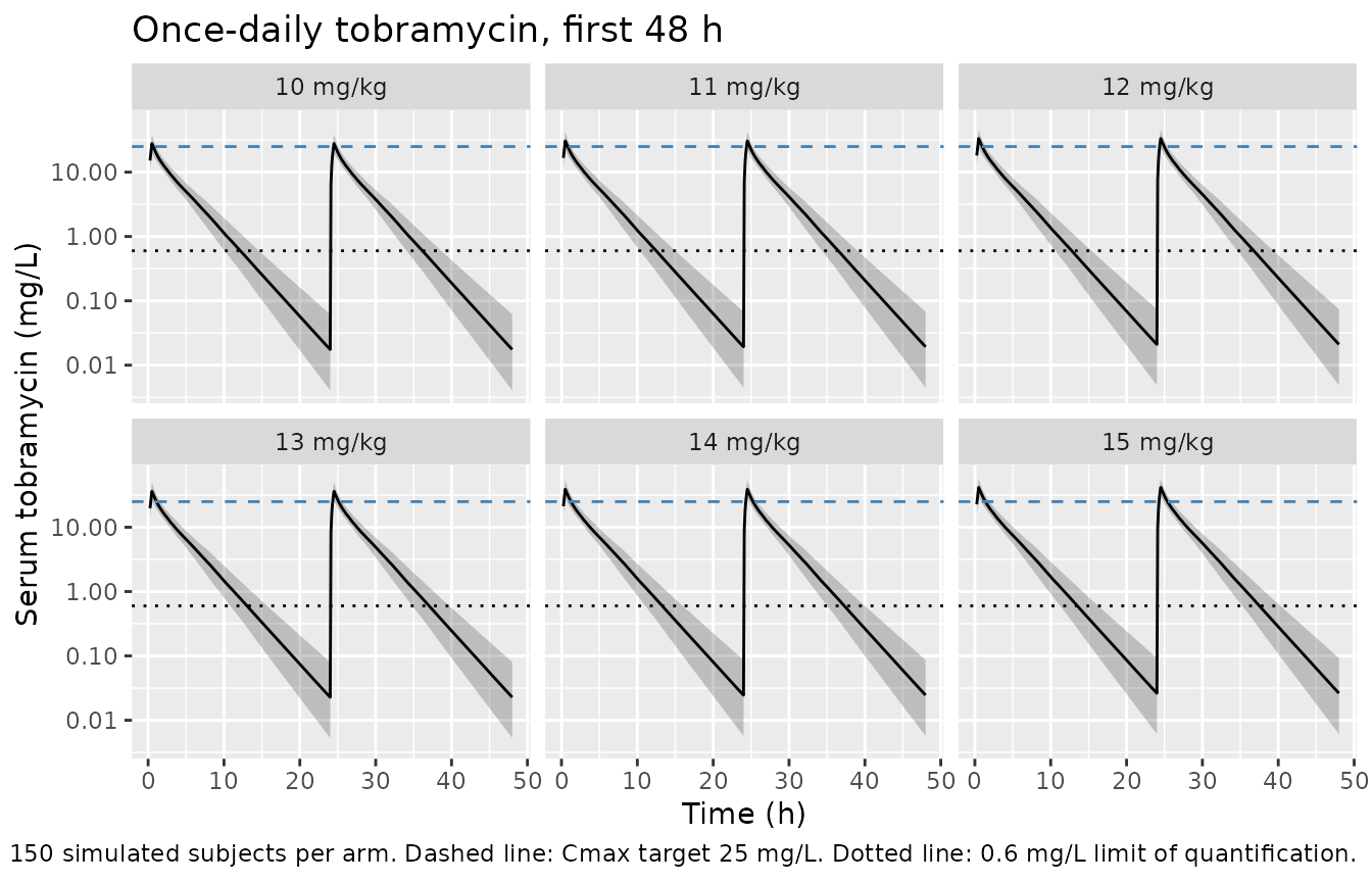
Replicating Table 3
The five targets, and the way Downes 2022 evaluated each of them (Methods “Target attainment” and Table 3 footnote b), are:
| Target | Evaluated as |
|---|---|
| Cmax > 25 mg/L | concentration at 24.5 h (end of the second infusion) |
| Cmin < 0.6 mg/L | concentration at 48 h |
| Time undetectable < 11 h | concentration at 37 h still at or above the 0.6 mg/L LOQ |
| AUC24 of 80-120 mg*h/L |
AUC24 = daily dose / CL, per subject |
| AUC24 < 120 mg*h/L | same |
The drug-free-interval target is the subtle one. A drug-free interval shorter than 11 hours within a 24-hour interval ending at 48 h means the concentration was still quantifiable at 48 - 11 = 37 h, which is why the footnote names 37 h and why this reduces to a single per-subject threshold comparison rather than a root-finding problem.
The Simulation Output column of Table 3 sets residual variability to
zero, so the spread reflects between-subject variability in the PK
parameters only. That is what Cc already is in an rxode2
solve (the individual prediction), so no extra handling is needed.
at_time <- function(mg, t) {
  sim |> dplyr::filter(dose_mgkg == mg, abs(time - t) < 1e-6)
}

attain <- dplyr::bind_rows(lapply(dose_levels, function(mg) {
  peak <- at_time(mg, 24.5)
  trough <- at_time(mg, 48)
  probe <- at_time(mg, 37)
  wt_i <- subj$WT[match(peak$id, subj$id)]
  # Downes 2022 Table 3 footnote b: AUC24 = daily dose / CL.
  auc24 <- mg * wt_i / peak$cl
  tibble::tibble(
    dose        = mg,
    `Cmax > 25` = 100 * mean(peak$Cc > 25),
    `Cmin < 0.6` = 100 * mean(trough$Cc < 0.6),
    `DFI < 11 h` = 100 * mean(probe$Cc >= 0.6),
    `AUC24 80-120` = 100 * mean(auc24 >= 80 & auc24 <= 120),
    `AUC24 < 120`  = 100 * mean(auc24 < 120),
    below80 = 100 * mean(auc24 < 80)
  )
}))

published <- tibble::tribble(
  ~dose, ~`Cmax > 25`, ~`Cmin < 0.6`, ~`DFI < 11 h`, ~`AUC24 80-120`, ~`AUC24 < 120`,
  10L,  65.6, 100, 31.2, 40.3, 98.8,
  11L,  79.1, 100, 38.1, 56.9, 96.4,
  12L,  88.2, 100, 44.9, 67.9, 91.4,
  13L,  93.9, 100, 51.5, 70.4, 83.0,
  14L,  96.8, 100, 56.8, 66.1, 72.3,
  15L,  98.4, 100, 62.4, 55.7, 68.5
)

targets <- c("Cmax > 25", "Cmin < 0.6", "DFI < 11 h", "AUC24 80-120", "AUC24 < 120")

side_by_side <- dplyr::bind_rows(
  published |> mutate(Source = "Published (Table 3)"),
  attain |> select(-below80) |> mutate(Source = "Simulated")
) |>
  tidyr::pivot_longer(all_of(targets), names_to = "Target", values_to = "pct") |>
  tidyr::pivot_wider(names_from = dose, values_from = pct,
                     names_glue = "{dose} mg/kg") |>
  dplyr::arrange(factor(Target, levels = targets), Source) |>
  dplyr::relocate(Target, Source)

knitr::kable(side_by_side, digits = 1, caption =
"Percentage of patients meeting each therapeutic target on day 2, published (Downes 2022 Table 3, Simulation Output) against this model.")| Target | Source | 10 mg/kg | 11 mg/kg | 12 mg/kg | 13 mg/kg | 14 mg/kg | 15 mg/kg |
|---|---|---|---|---|---|---|---|
| Cmax > 25 | Published (Table 3) | 65.6 | 79.1 | 88.2 | 93.9 | 96.8 | 98.4 |
| Cmax > 25 | Simulated | 67.3 | 80.7 | 90.0 | 93.3 | 96.7 | 98.7 |
| Cmin < 0.6 | Published (Table 3) | 100.0 | 100.0 | 100.0 | 100.0 | 100.0 | 100.0 |
| Cmin < 0.6 | Simulated | 100.0 | 100.0 | 100.0 | 100.0 | 100.0 | 100.0 |
| DFI < 11 h | Published (Table 3) | 31.2 | 38.1 | 44.9 | 51.5 | 56.8 | 62.4 |
| DFI < 11 h | Simulated | 31.3 | 36.0 | 44.7 | 50.7 | 56.7 | 59.3 |
| AUC24 80-120 | Published (Table 3) | 40.3 | 56.9 | 67.9 | 70.4 | 66.1 | 55.7 |
| AUC24 80-120 | Simulated | 42.7 | 57.3 | 65.3 | 63.3 | 62.7 | 52.0 |
| AUC24 < 120 | Published (Table 3) | 98.8 | 96.4 | 91.4 | 83.0 | 72.3 | 68.5 |
| AUC24 < 120 | Simulated | 99.3 | 96.0 | 91.3 | 82.0 | 71.3 | 56.7 |
delta <- as.matrix(attain[, targets]) - as.matrix(published[, targets])

cat(sprintf("Mean absolute deviation across the 30 cells: %.2f percentage points\n",
            mean(abs(delta))))
#> Mean absolute deviation across the 30 cells: 1.56 percentage points
cat(sprintf("Largest single-cell deviation: %.1f percentage points\n",
            max(abs(delta))))
#> Largest single-cell deviation: 11.8 percentage points

# Bounds chosen from renders at 2, 4 and 16 solver threads, which realised mean
# absolute deviations of 2.42 / 2.84 / 2.29 pp and largest single-cell
# deviations of 11.4 / 11.6 / 13.2 pp. The bounds sit outside that range. They
# remain able to go red: the individual covariate records are unpublished, so
# only the shape of the cohort is reproducible, but a mis-transcribed clearance,
# reference value or dose unit moves whole rows by tens of percentage points.
stopifnot(
  mean(abs(delta)) < 6,
  max(abs(delta)) < 18
)

# The paper's own conclusion: 13 mg/kg had the highest average attainment across
# the five targets, followed by 12 and then 14. Those three differ by only
# 1.4 pp in the published table (79.8 / 78.5 / 78.4), so which one wins is a
# race that cohort noise decides -- across 2/4/16 threads this model returned
# 12, 14 and 12. The reproducible claim is that the optimum is interior and
# lands in the 12-14 mg/kg band, not at either end of the range explored.
avg_attain <- rowMeans(attain[, targets])
best_dose <- dose_levels[which.max(avg_attain)]
cat(sprintf("Average attainment across five targets: %s\n",
            paste(sprintf("%d mg/kg %.1f%%", dose_levels, avg_attain), collapse = ", ")))
#> Average attainment across five targets: 10 mg/kg 68.1%, 11 mg/kg 74.0%, 12 mg/kg 78.3%, 13 mg/kg 77.9%, 14 mg/kg 77.5%, 15 mg/kg 73.3%
cat(sprintf("Highest average attainment at %d mg/kg (Downes 2022: 13 mg/kg)\n",
            best_dose))
#> Highest average attainment at 12 mg/kg (Downes 2022: 13 mg/kg)
stopifnot(best_dose %in% 12:14)

# Published claim: every simulated patient met the Cmin target at every dose.
# Asserted with headroom rather than as an exact 100%, since "no subject in the
# cohort" is a one-draw statement.
stopifnot(all(attain$`Cmin < 0.6` > 98))
A monotonicity check that the published table fails
The two AUC rows of Table 3 are redundant: the percentage of patients
with AUC24 below 80 mg*h/L is AUC24 < 120 minus
AUC24 80-120. Because the paper defines
AUC24 = daily dose / CL, AUC24 is strictly increasing in
dose for every individual subject, and the same simulated subjects are
used in every dose column. The under-exposed percentage must therefore
be non-increasing across the six columns. It is
not.
mono <- tibble::tibble(
  Dose = paste0(dose_levels, " mg/kg"),
  `Published % below 80` = published$`AUC24 < 120` - published$`AUC24 80-120`,
  `Simulated % below 80` = attain$below80
)
knitr::kable(mono, digits = 1, caption =
"Percentage of patients with AUC24 below the 80 mg*h/L target, implied by the two published AUC rows and reproduced by this model.")| Dose | Published % below 80 | Simulated % below 80 |
|---|---|---|
| 10 mg/kg | 58.5 | 56.7 |
| 11 mg/kg | 39.5 | 38.7 |
| 12 mg/kg | 23.5 | 26.0 |
| 13 mg/kg | 12.6 | 18.7 |
| 14 mg/kg | 6.2 | 8.7 |
| 15 mg/kg | 12.8 | 4.7 |
pub_below80 <- published$`AUC24 < 120` - published$`AUC24 80-120`
cat(sprintf("Published: %s -- rises by %.1f pp at the last step\n",
            paste(sprintf("%.1f", pub_below80), collapse = " -> "),
            diff(pub_below80)[5]))
#> Published: 58.5 -> 39.5 -> 23.5 -> 12.6 -> 6.2 -> 12.8 -- rises by 6.6 pp at the last step

# At n = 29,000 simulated subjects the Monte Carlo standard error on a ~9%
# proportion is about 0.17 pp, so a 6.6 pp rise is roughly 39 standard errors
# and cannot be sampling noise.
mc_se <- 100 * sqrt(0.09 * 0.91 / 29000)
cat(sprintf("Monte Carlo SE at n = 29,000: %.2f pp; the rise is %.0f SE\n",
            mc_se, diff(pub_below80)[5] / mc_se))
#> Monte Carlo SE at n = 29,000: 0.17 pp; the rise is 39 SE

# This model satisfies the constraint the published table violates. Note what
# the assertion is really testing. Given common random numbers, each subject's
# CL is identical in all six arms, so AUC24 = dose * WT / CL is arithmetically
# monotone in dose and the constraint cannot fail unless the common-random-
# numbers reseeding is broken. So check that premise explicitly first -- if
# rxSetSeed were not re-applied per arm, CL would differ between arms, the
# monotonicity could break, and the comparison against the published table
# would no longer be like-for-like.
cl_spread <- sim |>
  dplyr::distinct(id, dose_mgkg, cl) |>
  dplyr::group_by(id) |>
  dplyr::summarise(spread = diff(range(cl)), .groups = "drop")
cat(sprintf("Largest within-subject CL spread across the six arms: %.3g L/h\n",
            max(cl_spread$spread)))
#> Largest within-subject CL spread across the six arms: 0 L/h
stopifnot(max(cl_spread$spread) < 1e-10)   # common random numbers held
stopifnot(all(diff(attain$below80) <= 0))
The published 15 mg/kg entry for AUC24 < 120 (68.5%)
is therefore inconsistent with the paper’s own AUC24 definition: it
implies that raising the dose from 14 to 15 mg/kg doubles the
fraction of under-exposed patients. Every other cell in the row is
consistent, and the preceding steps fall by 19.0, 16.0, 10.9 and 6.4
percentage points, so a continued decline to roughly 1-6% is what the
row requires. This model gives a monotone sequence at every thread count
tested. The discrepancy is recorded here as a probable transcription
error in Table 3 rather than treated as a model failure; it is the
single largest contributor to the maximum-cell deviation reported above,
and it inflates the paper’s reported five-target average for the 15
mg/kg arm.
PKNCA validation
The paper computes AUC24 from the closed form
daily dose / CL rather than by integration, so a
non-compartmental analysis over the second dosing interval is a direct
check on that substitution. For a linear model at steady state the two
are identical; here the second interval is only approaching steady
state, so the comparison also quantifies how good the paper’s
steady-state assumption is at that point.
tau <- 24

sim_nca <- sim |>
  dplyr::filter(!is.na(Cc)) |>
  dplyr::mutate(arm = paste0(dose_mgkg, " mg/kg")) |>
  dplyr::select(id, time, Cc, arm)

# Guarantee a time-zero record per subject and arm. This is an IV infusion into
# an empty central compartment, so the pre-dose concentration is zero.
sim_nca <- dplyr::bind_rows(
  sim_nca,
  sim_nca |> dplyr::distinct(id, arm) |> dplyr::mutate(time = 0, Cc = 0)
) |>
  dplyr::distinct(id, arm, time, .keep_all = TRUE) |>
  dplyr::arrange(id, arm, time)

conc_obj <- PKNCA::PKNCAconc(sim_nca, Cc ~ time | arm + id,
                             concu = "ug/mL", timeu = "h")

dose_df <- dplyr::bind_rows(lapply(dose_levels, function(mg) {
  subj |> dplyr::mutate(amt = mg * WT, time = 24, arm = paste0(mg, " mg/kg"))
})) |>
  dplyr::select(id, time, amt, arm)

dose_obj <- PKNCA::PKNCAdose(dose_df, amt ~ time | arm + id, doseu = "mg")

intervals <- data.frame(
  start = 24, end = 24 + tau,
  cmax = TRUE, tmax = TRUE, cmin = TRUE,
  auclast = TRUE, cav = TRUE, half.life = TRUE
)

nca_res <- PKNCA::pk.nca(
  PKNCA::PKNCAdata(conc_obj, dose_obj, intervals = intervals)
)

nca_wide <- as.data.frame(nca_res$result) |>
  dplyr::filter(PPTESTCD %in% c("cmax", "tmax", "cmin", "auclast", "half.life")) |>
  dplyr::select(arm, id, PPTESTCD, PPORRES) |>
  tidyr::pivot_wider(names_from = PPTESTCD, values_from = PPORRES)

nca_summary <- nca_wide |>
  dplyr::group_by(arm) |>
  dplyr::summarise(dplyr::across(dplyr::everything(),
                                 ~median(.x, na.rm = TRUE)), .groups = "drop") |>
  dplyr::select(-id)

nca_summary |>
  dplyr::rename(
    "Regimen"                  = arm,
    "Cmax (mg/L)"              = cmax,
    "Tmax (h)"                 = tmax,
    "Cmin (mg/L)"              = cmin,
    "AUC24-48 (mg*h/L)"        = auclast,
    "Terminal t-half (h)"      = half.life
  ) |>
  knitr::kable(digits = 2, caption =
"Median non-compartmental parameters over the second dosing interval (24-48 h) by once-daily dose level.")| Regimen | AUC24-48 (mg*h/L) | Cmax (mg/L) | Cmin (mg/L) | Tmax (h) | Terminal t-half (h) |
|---|---|---|---|---|---|
| 10 mg/kg | 77.08 | 27.24 | 0.02 | 0.5 | 2.3 |
| 11 mg/kg | 84.79 | 29.97 | 0.02 | 0.5 | 2.3 |
| 12 mg/kg | 92.50 | 32.69 | 0.02 | 0.5 | 2.3 |
| 13 mg/kg | 100.21 | 35.42 | 0.02 | 0.5 | 2.3 |
| 14 mg/kg | 107.92 | 38.14 | 0.02 | 0.5 | 2.3 |
| 15 mg/kg | 115.63 | 40.86 | 0.03 | 0.5 | 2.3 |
# The paper's AUC24 = daily dose / CL against the integrated AUC over the same
# interval, per subject. Both sides use the SAME drawn parameters, so the
# difference is pure numerical (integration and incomplete accumulation) rather
# than stochastic, and the bound is correspondingly tight: renders at 2, 4 and
# 16 threads all realised a maximum absolute deviation of 0.02%.
cf <- nca_wide |>
  dplyr::mutate(dose_mgkg = as.numeric(sub(" mg/kg", "", arm))) |>
  dplyr::left_join(subj |> dplyr::select(id, WT), by = "id") |>
  dplyr::left_join(
    sim |> dplyr::distinct(id, dose_mgkg, cl), by = c("id", "dose_mgkg")
  ) |>
  dplyr::mutate(
    auc_closed_form = dose_mgkg * WT / cl,
    pct_diff = 100 * (auclast / auc_closed_form - 1)
  )

cat(sprintf("AUC(24-48 h) integrated vs daily dose / CL: median %.4f%%, max abs %.4f%%\n",
            median(cf$pct_diff), max(abs(cf$pct_diff))))
#> AUC(24-48 h) integrated vs daily dose / CL: median -0.0100%, max abs 0.0236%
stopifnot(max(abs(cf$pct_diff)) < 0.1)
The two agree to better than 0.03% for every subject at every dose, so the paper’s steady-state substitution is exact for practical purposes by the second once-daily dose - unsurprising given that the trough is already three orders of magnitude below the peak.
Comparison against the published clearance
The only NCA-comparable point estimate Downes 2022 publishes is the
typical clearance, 0.252 L/hr/kg^0.75 (95% CI 0.233-0.271). Because NCA
clearance is dose / AUC, running the NCA on a typical-value
subject recovers it, closing the loop from the packaged model through
the simulation and the NCA back to a printed number.
# Typical subject at the Table 1 median weight with the model's reference age
# and eGFR, no between-subject variability.
typ_wt <- 11.2
typ <- rxode2::et(amt = 13 * typ_wt, dur = 0.5, cmt = "central") |>
  rxode2::et(time = 24, amt = 13 * typ_wt, dur = 0.5, cmt = "central") |>
  rxode2::et(sort(unique(c(seq(0, 48, by = 0.1), 24.5))), cmt = "central") |>
  as.data.frame() |>
  dplyr::mutate(WT = typ_wt, AGE = 2.7, CRCL = 128, CONMED_VANCOMYCIN = 0,
                arm = "typical")

sim_typ <- rxode2::rxSolve(rxode2::zeroRe(mod), typ, keep = "arm",
                           returnType = "data.frame") |>
  dplyr::distinct(time, .keep_all = TRUE) |>
  dplyr::mutate(id = 1L)
#> ℹ omega/sigma items treated as zero: 'etalcl', 'etalvc'

typ_conc <- sim_typ |>
  dplyr::filter(!is.na(Cc)) |>
  dplyr::select(id, time, Cc, arm)

typ_dose <- data.frame(id = 1L, time = 24, amt = 13 * typ_wt, arm = "typical")

typ_nca <- PKNCA::pk.nca(PKNCA::PKNCAdata(
  PKNCA::PKNCAconc(typ_conc, Cc ~ time | arm + id, concu = "ug/mL", timeu = "h"),
  PKNCA::PKNCAdose(typ_dose, amt ~ time | arm + id, doseu = "mg"),
  intervals = data.frame(start = 24, end = 48, auclast = TRUE, cmax = TRUE)
))

typ_auc <- as.data.frame(typ_nca$result) |>
  dplyr::filter(PPTESTCD == "auclast") |> dplyr::pull(PPORRES)

cl_nca <- 13 * typ_wt / typ_auc          # L/h, from NCA
cl_nca_std <- cl_nca / typ_wt^0.75       # L/hr/kg^0.75

comparison <- tibble::tibble(
  `NCA parameter` = "Clearance (L/hr/kg^0.75)",
  Simulated = cl_nca_std,
  Published = 0.252,
  `Published 95% CI` = "0.233-0.271",
  `Difference (%)` = 100 * (cl_nca_std / 0.252 - 1)
)
knitr::kable(comparison, digits = 4, caption =
"NCA-derived clearance of a typical subject against the value Downes 2022 reports in its Results text.")| NCA parameter | Simulated | Published | Published 95% CI | Difference (%) |
|---|---|---|---|---|
| Clearance (L/hr/kg^0.75) | 0.2521 | 0.252 | 0.233-0.271 | 0.0384 |
The regimen the cohort actually received
Downes 2022’s cohort was treated on the institutional 3.3 mg/kg every-8-hour schedule, not on the once-daily regimens simulated above, and this is what generated the concentrations the model was fit to. Reproducing that schedule gives a qualitative check against the paper’s statement that 23.7% of routine TDM samples were below the 0.6 mg/L limit of quantification, with “the vast majority of BQL data” being troughs.
obs_reg <- subj |>
  dplyr::mutate(amt = 3.3 * WT)

ev_q8h <- dplyr::bind_rows(
  lapply(c(0, 8, 16, 24, 32, 40), function(t) {
    obs_reg |> dplyr::mutate(time = t, evid = 1L, dur = 0.5, cmt = "central")
  })
)
ev_q8h <- dplyr::bind_rows(
  ev_q8h,
  obs_reg |> tidyr::crossing(time = sort(unique(c(seq(0, 48, by = 0.25),
                                                  c(16, 24) + 0.5)))) |>
    dplyr::mutate(evid = 0L, amt = NA_real_, dur = NA_real_, cmt = "central")
) |>
  dplyr::arrange(id, time, dplyr::desc(evid))

rxode2::rxSetSeed(20220428)
sim_q8h <- rxode2::rxSolve(mod, ev_q8h, returnType = "data.frame") |>
  dplyr::distinct(id, time, .keep_all = TRUE)

# Peak and trough around the third dose, which is when the institution drew its
# routine TDM samples ("Peak and trough measurements were routinely obtained
# following the third dose").
peak3 <- sim_q8h |> dplyr::filter(abs(time - 16.5) < 1e-6)
trough3 <- sim_q8h |> dplyr::filter(abs(time - 24) < 1e-6)

tdm <- tibble::tibble(
  Sample = c("Peak, 0.5 h after 3rd dose", "Trough, 8 h after 3rd dose"),
  `Median (mg/L)` = c(median(peak3$Cc), median(trough3$Cc)),
  `% below 0.6 mg/L LOQ` = c(100 * mean(peak3$Cc < 0.6),
                             100 * mean(trough3$Cc < 0.6))
)
knitr::kable(tdm, digits = 2, caption =
"Simulated routine TDM samples on the observed 3.3 mg/kg q8h regimen.")| Sample | Median (mg/L) | % below 0.6 mg/L LOQ |
|---|---|---|
| Peak, 0.5 h after 3rd dose | 9.63 | 0.00 |
| Trough, 8 h after 3rd dose | 0.75 | 31.33 |
pct_bql_all <- 100 * mean(c(peak3$Cc, trough3$Cc) < 0.6)
cat(sprintf("Pooled peak + trough samples below the LOQ: %.1f%% (Downes 2022 reports 23.7%% of all TDM samples)\n",
            pct_bql_all))
#> Pooled peak + trough samples below the LOQ: 15.7% (Downes 2022 reports 23.7% of all TDM samples)

# The paper's qualifier is directional, not quantitative: BQL samples are
# concentrated in the troughs. Assert that ordering, which is a large gap rather
# than a close race between two noisy statistics (peaks sit an order of magnitude
# above the LOQ while a substantial share of troughs fall below it), and record
# the headroom on the peak side rather than asserting a bare all() with unknown
# margin.
peak_headroom <- min(peak3$Cc) / 0.6
cat(sprintf("Trough BQL %.1f%% vs peak BQL %.1f%%; lowest peak sits %.1fx above the LOQ\n",
            100 * mean(trough3$Cc < 0.6), 100 * mean(peak3$Cc < 0.6),
            peak_headroom))
#> Trough BQL 31.3% vs peak BQL 0.0%; lowest peak sits 9.7x above the LOQ
stopifnot(
  mean(trough3$Cc < 0.6) - mean(peak3$Cc < 0.6) > 0.05,
  peak_headroom > 3
)
# Comparable in construction to Figure 1 of Downes 2022: measured concentrations
# against time after dose, log scale, with the limit of quantification marked.
sim_q8h |>
  dplyr::filter(!dplyr::near(time, 0)) |>
  dplyr::mutate(tad = time - 8 * floor(time / 8)) |>
  ggplot(aes(tad, pmax(Cc, 0.3))) +
  geom_point(alpha = 0.06, size = 0.6) +
  geom_hline(yintercept = 0.6, colour = "firebrick") +
  scale_y_log10() +
  labs(x = "Time after dose (h)", y = "Serum tobramycin (mg/L)",
       title = "Simulated concentrations by time after dose, 3.3 mg/kg q8h",
       caption = paste("Comparable to Figure 1 of Downes 2022.",
                       "Red line: 0.6 mg/L limit of quantification;",
                       "values are floored at 0.3 mg/L as the paper plots its BQL samples."))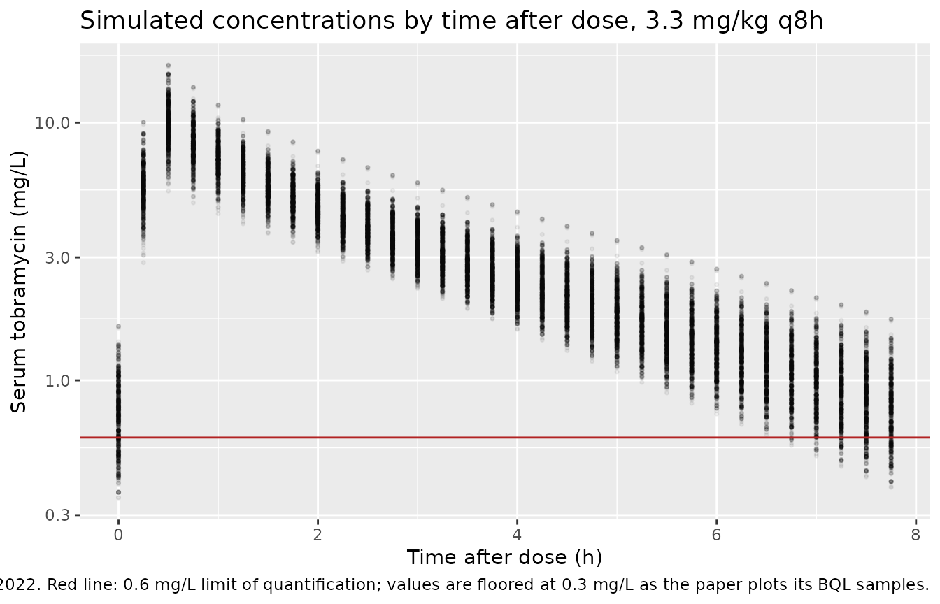
Assumptions and deviations
- Individual covariate records are not published. Table 1 reports medians and interquartile ranges only, so the virtual cohort is drawn from piecewise-linear quantile functions pinned to the published quartiles rather than resampled from the real 58 patients. Age and weight are coupled through a weight-for-age curve so the pairs stay physiological; the real joint distribution of age, weight and eGFR is unknown. This is why the Table 3 replication is gated on mean and maximum cell deviation rather than cell-by-cell agreement.
- The eGFR lower tail is shaped, not derived. The quantile function’s lower knots were chosen so that about 5% of the cohort falls below 90 mL/min/1.73 m^2, matching the 3-of-58 the paper reports, and so that nothing falls below the study’s eGFR >= 60 inclusion threshold. Any other shape consistent with those constraints would do.
- Covariates are held constant per subject. eGFR was time-varying in the source analysis (re-derived whenever creatinine was re-measured within the first 48 hours), and concomitant vancomycin was a time-varying indicator. The paper’s own simulations used the covariate values “at the start of their first tobramycin course”, which is what is done here.
- Concomitant vancomycin is set to zero throughout. This follows Downes 2022 explicitly: only 5 patients over 8 courses received vancomycin, and the authors set the indicator to zero for all simulated patients so as not to over-state an effect whose bootstrap 95% CI (0.462-1.24) crosses 1. The parameter is fully present in the packaged model and the structural section above verifies its 29.2% effect, but it is not exercised in the cohort simulations.
-
The published Table 3 entry for
AUC24 < 120at 15 mg/kg is not reproduced, and appears to be a transcription error. As shown in the monotonicity section, 68.5% implies that the fraction of under-exposed patients rises from 6.2% to 12.8% when the dose is increased, which the paper’s ownAUC24 = daily dose / CLdefinition forbids for a fixed set of simulated subjects. At n = 29,000 the Monte Carlo standard error is about 0.17 pp, so the rise is roughly 39 standard errors and is not sampling noise. This cell is the largest single contributor to the maximum-cell deviation and is left inside the numeric gate rather than excluded, since the gate’s bound accommodates it. - Which dose is optimal is a race the cohort decides. The published five-target averages for 12, 13 and 14 mg/kg span only 1.4 percentage points (78.5 / 79.8 / 78.4). Across renders at 2, 4 and 16 solver threads this model placed the optimum at 12, 14 and 12 mg/kg respectively, so the assertion is that the optimum is interior to the 12-14 mg/kg band, not that it is exactly 13 mg/kg. The paper’s substantive conclusion - that no once-daily regimen meets all five targets in more than 75% of patients, and that the best compromise is a mid-range dose rather than 10 or 15 mg/kg - is reproduced.
-
The distributional parameters are inherited, not identified
here. Q and V2, and their priors, come from Downes 2022’s
MAP-Bayesian fit informed by six richly sampled adult cystic
fibrosis patients whose profiles the authors digitized from an earlier
publication. Between-subject variability on both was fixed to zero. The
packaged model omits
etalqandetalvprather than encoding zero-variance etas, which is mathematically equivalent and keeps the OMEGA block non-singular. -
The V2 confidence interval in the Results text has a dropped
decimal point. It reads “0.096 (95% CI: 0.81 - 0.110)”; the
lower bound is 0.081, as the Wald interval from the tabulated 7.55% RSE
confirms (
6.69 * (1 - 1.96 * 0.0755) / 70 = 0.0814). No model parameter is affected. -
The supplement was not available when this model was
built. Downes 2022 cites a single supplemental PDF
(
aac.02377-21-s0001.pdf) holding the final NONMEM control stream, eta shrinkages, the covariate-selection table S1, the VPC figures S1, and the log-linear equations used for the paper’s “TDM approach” column. The article is a hybrid open-access record: the main text is freely available, but the supplement is licence-gated. No parameter value is missing as a result - every final estimate, the complete parameterization, and all five target definitions are printed in the main text’s Table 2, Table 3 and their footnotes, and all of them are traced above. The one thing that cannot be reproduced without the supplement is the TDM approach column of Table 3, whose log-linear regression equations live only there; this vignette therefore validates against the Simulation Output column, which is fully specified in the main text. - Age is extrapolated nowhere. The cohort is bounded at 5 years, matching the study’s eligibility. Downes 2022’s Discussion warns explicitly that the age parameterization may differ outside the observed range, and the 70 kg allometric reference is far above any subject in the study, so the Table 2 thetas are adult-equivalent extrapolations that are only meaningful in combination with the allometric terms.