Venetoclax with R-CHOP in non-Hodgkin lymphoma (Samineni 2022)
Source:vignettes/articles/Samineni_2022_venetoclax.Rmd
Samineni_2022_venetoclax.RmdModel and source
- Citation: Samineni D, Huang W, Gibiansky L, Ding H, Zhang R, Li C, Sinha A, Rajwanshi R, Humphrey K, Bazeos A, Salem AH, Miles D. Population Pharmacokinetics and Exposure-Response Analyses for Venetoclax in Combination with R-CHOP in Relapsed/Refractory and Previously Untreated Patients with Diffuse Large B Cell Lymphoma. Adv Ther. 2022;39(1):598-618. doi:10.1007/s12325-021-01919-z. Parameter values from Table 2; the legacy model is Jones AK et al., AAPS J 2016;18(5):1192-1202, doi:10.1208/s12248-016-9927-9.
- Description: Two-compartment population PK model with first-order absorption and first-order elimination for oral venetoclax given with R-CHOP to adults with relapsed/refractory or previously untreated non-Hodgkin lymphoma, mostly diffuse large B-cell lymphoma (the phase 1b/2 CAVALLI study, GO27878). Every structural, covariate, random-effect and residual value is carried FIXED from the legacy venetoclax population PK model (505 subjects with CLL/SLL, NHL and healthy volunteers); Samineni 2022 estimated only the two multiplicative CAVALLI study effects, x1.63 on CL/F and x2.33 on V2/F. Relative bioavailability depends on the meal (fasting / low-fat reference / moderate-fat / high-fat / fed with the meal unspecified) and on a fixed power function of the dose (reference 400 mg). CL/F is lowered by strong and moderate CYP3A inhibitors and by OATP1B3 inhibitors; V2/F is higher in patients than in healthy volunteers and lower in women. Log-normal IIV on CL/F, V2/F and F1; combined proportional and additive residual error. Eight companion exposure-response logistic models in the Samineni_2022_venetoclax_* family take the steady-state nominal-dose AUC derived from this model as an input column.
- Article: https://doi.org/10.1007/s12325-021-01919-z (open access; PMC8799559)
Samineni et al. analysed venetoclax pharmacokinetics (PK) and exposure-response in CAVALLI (GO27878), a phase 1b/2 study of venetoclax with rituximab plus cyclophosphamide, doxorubicin, vincristine and prednisone (R-CHOP) in non-Hodgkin lymphoma. The paper is in two parts.
-
Population PK. The legacy venetoclax population PK
model, fitted to 505 subjects in eight earlier studies, was applied to
the CAVALLI data with every parameter held at its prior estimate. A
multiplicative CAVALLI study effect was then estimated on apparent
clearance (x1.63) and on apparent central volume (x2.33). Table 2
reprints every value, so the whole model is packaged here as
Samineni_2022_venetoclax. -
Exposure-response. Individual post hoc PK
parameters gave a steady-state nominal-dose exposure,
AUCss nominal = Dnom * F1 / (CL/F)(Eq. 1). This exposure was related to five grade >= 3 safety endpoints (Table 4, Figure 5) and to complete response by PET-CT at the end of treatment (Figure 4). Cox models related it to progression-free survival (Table 3).
The exposure-response regressions are packaged as thirteen companion models.
| Model | Endpoint | Source of the coefficients |
|---|---|---|
Samineni_2022_venetoclax_neutropenia |
grade >= 3 neutropenia | Table 4 |
Samineni_2022_venetoclax_infection |
grade >= 3 infections | Table 4 (with age) |
Samineni_2022_venetoclax_febrile_neutropenia |
grade >= 3 febrile neutropenia | Table 4 (with IPI 4-5) |
Samineni_2022_venetoclax_thrombocytopenia |
grade >= 3 thrombocytopenia | Table 4 (with age and ECOG >= 2) |
Samineni_2022_venetoclax_sae |
serious adverse events | Table 4 (with age) |
Samineni_2022_venetoclax_<endpoint>_base (five
files) |
the same five endpoints | Figure 5 fitted curve, digitised |
Samineni_2022_venetoclax_petcr |
PET-CT complete response, all-comers | Figure 4a, digitised |
Samineni_2022_venetoclax_petcr_bcl2_fish |
PET-CT complete response by BCL-2 FISH | Figure 4b, digitised |
Samineni_2022_venetoclax_petcr_bcl2_ihc |
PET-CT complete response by BCL-2 IHC | Figure 4c, digitised |
Why the Figure 5 curves are packaged separately from Table 4 is explained in Table 4 and Figure 5 disagree.
Population
The PK analysis covered 232 CAVALLI patients (Table 1): median age 64 years (range 18-85), median weight 77.0 kg (46.0-182), 44.4% women, 71.1% White and 23.7% race unknown. Most had diffuse large B-cell lymphoma (DLBCL; 94.0%), and the rest follicular, transformed or other lymphoma. Venetoclax was given once daily on days 4-10 of cycle 1 and days 1-10 of cycles 2-8 of 21-day cycles, mostly at 800 mg (214 patients; 200, 400 and 600 mg in 7, 3 and 8). Among CYP3A inhibitors, 66.7% of patients received weak ones only, 28.5% a moderate but no strong one, and 2.6% a strong one. 1.3% received an OATP1B3 inhibitor.
The exposure-safety analysis used 216 patients in phase 1b and phase 2 dosed at 400 (n = 3), 600 (n = 8) or 800 mg (n = 205). The exposure-efficacy analysis used 199 phase 2 patients with previously untreated DLBCL at 800 mg. Of these, 101 were BCL-2 IHC high and 40 were BCL-2 FISH positive.
Source trace
Every ini() value carries an in-file source comment. The
table collects them.
| Parameter / equation | Value | Source location |
|---|---|---|
| CL/F | 447 L/day, fixed | Table 2 |
| V2/F | 118 L, fixed | Table 2 |
| Q/F | 97.2 L/day, fixed | Table 2 |
| V3/F | 119 L, fixed | Table 2 |
| ka | 3.72 1/day, fixed | Table 2 |
| CL/F factor, strong / moderate CYP3A inhibitor | 0.18 / 0.84, fixed | Table 2 |
| CL/F factor, OATP1B3 inhibitor | 0.85, fixed | Table 2 |
| CL/F factor, GO27878 (CAVALLI) | 1.63 (95% CI 1.49-1.76), estimated | Table 2; Results |
| V2/F factor, CLL/SLL/NHL patient | 1.71, fixed | Table 2 |
| V2/F factor, female | 0.68, fixed | Table 2 |
| V2/F factor, GO27878 (CAVALLI) | 2.33 (95% CI 2.17-2.54), estimated | Table 2; Results |
| F1 factor, fasting / moderate fat / high fat / fed | 0.34 / 1.31 / 1.43 / 1.23 (low fat = 1), fixed | Table 2 |
| F1 dose exponent, (DOSE / 400)^theta | -0.18, fixed | Table 2 |
| omega^2 CL/F, V2/F, F1 | 0.15, 0.21, 0.10, fixed | Table 2 |
| sigma^2 proportional, additive | 0.22, 3.07e-7 (mg/L)^2, fixed | Table 2 |
| t1/2 check | 1.05 day | Table 2 |
| Exposure metric | AUCss nominal = Dnom * F1 / (CL/F) | Eq. 1 |
| Safety logistic coefficients | intercept, AUC slope, covariates | Table 4 |
| Safety drawn curves | intercept, AUC slope | Figure 5a-e, digitised |
| PET-CR curves | intercept, AUC slope per stratum | Figure 4a-c, digitised |
Population PK model
Virtual CAVALLI cohort
A cohort of 200 patients is built from the Table 1 distributions. Everyone is on 800 mg, the CAVALLI study effect is on, and doses follow the protocol low-fat meal.
mod <- rxode2::rxode(readModelDb("Samineni_2022_venetoclax"))
#> ℹ parameter labels from comments will be replaced by 'label()'

set.seed(2022)
n_sub <- 200
cyp <- sample(c("none", "weak", "moderate", "strong"), n_sub, replace = TRUE,
              prob = c(5, 152, 65, 6))
cohort <- data.frame(
  id = seq_len(n_sub),
  SEXF = rbinom(n_sub, 1, 0.444),
  CONMED_CYP3A4_INH_MOD = as.integer(cyp == "moderate"),
  CONMED_CYP3A4_INH_STRONG = as.integer(cyp == "strong"),
  CONMED_OATP1B_INH = rbinom(n_sub, 1, 0.013),
  STUDY_CAVALLI = 1,
  DIS_HEALTHY = 0,
  FED = 1, FED_LOWFAT = 1, FED_MEDFAT = 0, FED_HIGHFAT = 0,
  DOSE = 800,
  treatment = "800 mg QD"
)

# Ten once-daily doses (one 10-day cycle block), observed every 0.05 day.
ev_one <- rxode2::et(amt = 800, ii = 1, addl = 9, cmt = "depot") |>
  rxode2::et(seq(0, 10, by = 0.05), cmt = "central") |>
  as.data.frame()
ev_one$id <- NULL
events <- merge(cohort, ev_one, by = NULL) |>
  dplyr::arrange(id, time, dplyr::desc(evid)) |>
  # Event columns first: a DOSE covariate placed before amt is read as the amount.
dplyr::relocate(id, time, evid, cmt, amt, ii, addl)Concentration-time profiles
sim |>
  dplyr::group_by(time) |>
  dplyr::summarise(p05 = quantile(Cc, 0.05), p50 = median(Cc),
                   p95 = quantile(Cc, 0.95), .groups = "drop") |>
  ggplot2::ggplot(ggplot2::aes(time, p50)) +
  ggplot2::geom_ribbon(ggplot2::aes(ymin = p05, ymax = p95), alpha = 0.25) +
  ggplot2::geom_line() +
  ggplot2::labs(x = "Time (day)", y = "Venetoclax concentration (ug/mL)") +
  ggplot2::theme_bw()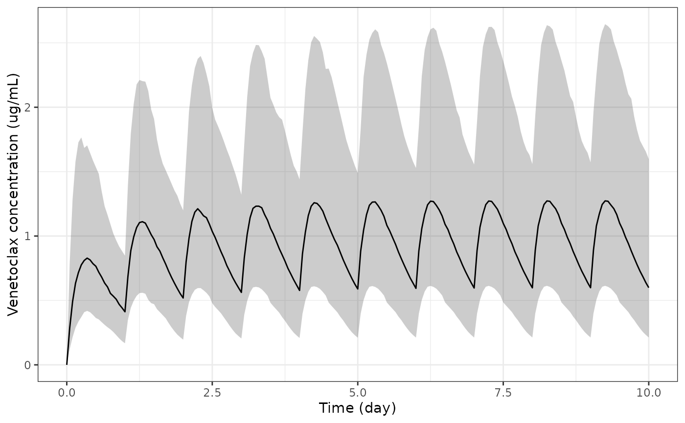
Simulated venetoclax concentrations over a 10-day block of 800 mg once daily in the virtual CAVALLI cohort: median and 5th-95th percentiles. Compare the spread with the observed concentrations in Figure 1 of Samineni 2022.
Structural checks
Table 2 prints a terminal half-life of 1.05 day. For a typical CAVALLI man it follows from the two-compartment eigenvalues, with no simulation involved.
p <- mod$theta
cl <- exp(p[["lcl"]]) * p[["e_study_cavalli_cl"]]
vc <- exp(p[["lvc"]]) * p[["e_dis_patient_vc"]] * p[["e_study_cavalli_vc"]]
q  <- exp(p[["lq"]]); vp <- exp(p[["lvp"]])
k10 <- cl / vc; k12 <- q / vc; k21 <- q / vp
beta <- ((k10 + k12 + k21) - sqrt((k10 + k12 + k21)^2 - 4 * k10 * k21)) / 2
t_half <- log(2) / beta
stopifnot(round(t_half, 2) == 1.05)
t_half
#> [1] 1.046335
The individual steady-state AUC over day 9-10 should equal Eq. 1,
DOSE * F1 / (CL/F), from the same drawn parameters. Both
sides use the same etas, so the only difference is how far the profile
is from steady state on day 9 and the trapezoidal error.
auc_trap <- sim |>
  dplyr::filter(time >= 9, time <= 10) |>
  dplyr::group_by(id) |>
  dplyr::summarise(auc_day10 = sum(diff(time) * (head(Cc, -1) + tail(Cc, -1)) / 2),
                   .groups = "drop")
indiv <- sim |>
  dplyr::group_by(id) |>
  dplyr::slice(1) |>
  dplyr::ungroup() |>
  dplyr::transmute(id, cl, fdepot, DOSE, auc_eq1 = DOSE * fdepot / cl) |>
  dplyr::left_join(auc_trap, by = "id")

ratio <- indiv$auc_day10 / indiv$auc_eq1
stopifnot(
  # Centre: steady state is reached by day 9 for nearly everyone.
  abs(median(ratio) - 1) < 0.01,
  # Envelope: a few strong-inhibitor patients with long half-lives are not yet
  # at steady state, so the tail is checked at a robust quantile.
  quantile(ratio, 0.1) > 0.95
)
summary(ratio)
#>    Min. 1st Qu.  Median    Mean 3rd Qu.    Max.
#>  0.5540  0.9970  0.9978  0.9926  0.9982  0.9986
Covariate effects
The food and dose effects on F1 are checked on typical values
(zeroRe()) by reading back the fdepot the
model computes for each meal level.
mod_typ <- rxode2::zeroRe(mod)
meals <- data.frame(
  meal = c("fasting", "low fat", "moderate fat", "high fat", "fed, unspecified"),
  FED = c(0, 1, 1, 1, 1), FED_LOWFAT = c(0, 1, 0, 0, 0),
  FED_MEDFAT = c(0, 0, 1, 0, 0), FED_HIGHFAT = c(0, 0, 0, 1, 0)
)
meal_ev <- meals |>
  dplyr::mutate(id = dplyr::row_number(), time = 0, evid = 1L, cmt = "depot",
                amt = 400, SEXF = 0, CONMED_CYP3A4_INH_MOD = 0,
                CONMED_CYP3A4_INH_STRONG = 0, CONMED_OATP1B_INH = 0,
                STUDY_CAVALLI = 1, DIS_HEALTHY = 0, DOSE = 400) |>
  dplyr::bind_rows(
    meals |>
      dplyr::mutate(id = dplyr::row_number(), time = 1, evid = 0L, cmt = "central",
                    amt = NA_real_, SEXF = 0, CONMED_CYP3A4_INH_MOD = 0,
                    CONMED_CYP3A4_INH_STRONG = 0, CONMED_OATP1B_INH = 0,
                    STUDY_CAVALLI = 1, DIS_HEALTHY = 0, DOSE = 400)
  ) |>
  dplyr::arrange(id, time) |>
  dplyr::relocate(id, time, evid, cmt, amt)
meal_sim <- rxode2::rxSolve(mod_typ, meal_ev, returnType = "data.frame")
#> ℹ omega/sigma items treated as zero: 'etalcl', 'etalvc', 'etalfdepot'
#> Warning: multi-subject simulation without without 'omega'
f_meal <- meal_sim |> dplyr::group_by(id) |> dplyr::slice(1) |> dplyr::pull(fdepot)
stopifnot(isTRUE(all.equal(f_meal, c(0.34, 1, 1.31, 1.43, 1.23))))

dose_f <- (c(200, 400, 600, 800) / 400)^p[["e_dose_fdepot"]]
data.frame(Meal = meals$meal, `F1 factor` = f_meal, check.names = FALSE) |>
knitr::kable(caption = "Typical F1 by meal at 400 mg, reproducing Table 2.")| Meal | F1 factor |
|---|---|
| fasting | 0.34 |
| low fat | 1.00 |
| moderate fat | 1.31 |
| high fat | 1.43 |
| fed, unspecified | 1.23 |
data.frame(`Dose (mg)` = c(200, 400, 600, 800), `F1 factor` = signif(dose_f, 3),
           check.names = FALSE) |>
knitr::kable(caption = "Dose nonlinearity on F1, (DOSE / 400)^-0.18.")| Dose (mg) | F1 factor |
|---|---|
| 200 | 1.130 |
| 400 | 1.000 |
| 600 | 0.930 |
| 800 | 0.883 |
PKNCA
PKNCA is run on the day 9-10 steady-state interval of the cohort. A typical 800 mg single dose followed for 10 days gives the terminal half-life.
conc_ss <- sim |>
  dplyr::filter(!is.na(Cc)) |>
  dplyr::select(id, time, Cc, treatment)
# One record per administered dose (the event table used addl).
dose_ss <- expand.grid(id = cohort$id, time = 0:9) |>
  dplyr::mutate(amt = 800, treatment = "800 mg QD")

res_ss <- PKNCA::pk.nca(PKNCA::PKNCAdata(
  PKNCA::PKNCAconc(conc_ss, Cc ~ time | treatment + id),
  PKNCA::PKNCAdose(dose_ss, amt ~ time | treatment + id),
  intervals = data.frame(start = 9, end = 10, cmax = TRUE, tmax = TRUE,
                         auclast = TRUE, cav = TRUE)
))

# Typical-value single dose for the terminal half-life.
sd_ev <- rxode2::et(amt = 800, cmt = "depot") |>
  rxode2::et(seq(0, 10, by = 0.05), cmt = "central") |>
  as.data.frame() |>
  dplyr::mutate(SEXF = 0, CONMED_CYP3A4_INH_MOD = 0, CONMED_CYP3A4_INH_STRONG = 0,
                CONMED_OATP1B_INH = 0, STUDY_CAVALLI = 1, DIS_HEALTHY = 0,
                FED = 1, FED_LOWFAT = 1, FED_MEDFAT = 0, FED_HIGHFAT = 0,
                DOSE = 800, treatment = "800 mg single dose, typical male")
sd_sim <- rxode2::rxSolve(mod_typ, sd_ev, returnType = "data.frame",
                          keep = "treatment") |>
  dplyr::mutate(id = 1L)
#> ℹ omega/sigma items treated as zero: 'etalcl', 'etalvc', 'etalfdepot'
res_sd <- PKNCA::pk.nca(PKNCA::PKNCAdata(
  PKNCA::PKNCAconc(dplyr::filter(sd_sim, !is.na(Cc)), Cc ~ time | treatment + id),
  PKNCA::PKNCAdose(data.frame(id = 1L, time = 0, amt = 800,
                              treatment = "800 mg single dose, typical male"),
                   amt ~ time | treatment + id),
  intervals = data.frame(start = 0, end = Inf, cmax = TRUE, tmax = TRUE,
                         half.life = TRUE)
))

as.data.frame(res_ss$result) |>
  dplyr::filter(PPTESTCD %in% c("cmax", "tmax", "auclast", "cav")) |>
  dplyr::group_by(treatment, PPTESTCD) |>
  dplyr::summarise(median = signif(median(PPORRES), 3),
                   p05 = signif(quantile(PPORRES, 0.05), 3),
                   p95 = signif(quantile(PPORRES, 0.95), 3), .groups = "drop") |>
knitr::kable(caption = "Steady-state NCA over day 9-10 (concentration in ug/mL, time in day).")| treatment | PPTESTCD | median | p05 | p95 |
|---|---|---|---|---|
| 800 mg QD | auclast | 0.984 | 0.439 | 2.13 |
| 800 mg QD | cav | 0.984 | 0.439 | 2.13 |
| 800 mg QD | cmax | 1.280 | 0.617 | 2.67 |
| 800 mg QD | tmax | 0.300 | 0.200 | 0.35 |
Comparison against published NCA
Samineni 2022 reports no NCA. The only PK summary it prints is the 1.05-day half-life in Table 2.
published <- data.frame(treatment = "800 mg single dose, typical male",
                        half.life = 1.05)
cmp <- nlmixr2lib::ncaComparisonTable(res_sd, published, by = "treatment",
                                      params = "half.life",
                                      units = c(half.life = "day"))
knitr::kable(cmp, caption = "Terminal half-life against Table 2.")| NCA parameter | treatment | Reference | Simulated | % diff |
|---|---|---|---|---|
| t½ (day) | 800 mg single dose, typical male | 1.05 | 1.03 | -1.5% |
hl_sim <- as.data.frame(res_sd$result) |>
  dplyr::filter(PPTESTCD == "half.life") |>
  dplyr::pull(PPORRES)
# Typical-value solve: the only difference from the eigenvalue half-life is
# how much of the distribution phase the lambda-z window still contains.
stopifnot(abs(hl_sim / 1.05 - 1) < 0.05)
Exposure scale: Eq. 1 against the paper’s exposure axis
The exposure-response models take AUC_VENETOCLAX_SS,
which Eq. 1 computes from the individual CL/F and F1. Applied to the
packaged model and the CAVALLI-like cohort, Eq. 1 gives the distribution
below. The paper’s own exposure axis (Figures 4 and 5) has quartile
bounds near 0.43, 0.55 and 0.68 ug*day/mL.
paper_q <- c(`25%` = 0.43, `50%` = 0.55, `75%` = 0.68)
sim_q <- quantile(indiv$auc_eq1, c(0.25, 0.5, 0.75))
data.frame(Quantile = names(paper_q), `Eq. 1 on Table 2` = signif(sim_q, 3),
           `Paper axis` = paper_q, Ratio = signif(sim_q / paper_q, 3),
           check.names = FALSE, row.names = NULL) |>
knitr::kable(caption = "Eq. 1 exposures from the packaged PK model against the paper's exposure-quartile bounds.")| Quantile | Eq. 1 on Table 2 | Paper axis | Ratio |
|---|---|---|---|
| 25% | 0.727 | 0.43 | 1.69 |
| 50% | 0.986 | 0.55 | 1.79 |
| 75% | 1.380 | 0.68 | 2.04 |
The model’s median is about 1.8-fold above the paper’s. Typical values account for most of it: a man on a weak inhibitor gets 800 x 0.883 / (447 x 1.63) = 0.97 ug*day/mL. No quantity printed in the paper explains the gap. The 10/21-day schedule would scale a cycle-averaged AUC by 0.48, close to but not equal to the observed ratio, and the paper defines the metric as a steady-state daily AUC without such a factor. The PK model is shipped as printed. The consequences for chaining it into the exposure-response models are shown at the end.
Exposure-response models
All thirteen are static logistic models: the exposure enters as a data column and there is no time dimension. Each model is evaluated by solving it over a data frame of covariate values.
er_names <- c(
  "neutropenia", "infection", "febrile_neutropenia", "thrombocytopenia", "sae",
  "neutropenia_base", "infection_base", "febrile_neutropenia_base",
  "thrombocytopenia_base", "sae_base",
  "petcr", "petcr_bcl2_fish", "petcr_bcl2_ihc"
)
er_ui <- lapply(er_names, function(nm) {
  rxode2::rxode(readModelDb(paste0("Samineni_2022_venetoclax_", nm)))
})
names(er_ui) <- er_names

solve_er <- function(nm, covs) {
  ev <- data.frame(id = seq_len(nrow(covs)), time = 0, evid = 0L)
  ev <- cbind(ev, covs)
  out <- rxode2::rxSolve(er_ui[[nm]], ev, returnType = "data.frame")
  out[[grep("^prob_", names(out), value = TRUE)[1]]]
}

er_ui[["thrombocytopenia"]]$theta
#>                          logit_ref                        e_auc_logit
#>                             -8.700                              0.590
#>                        e_age_logit                   e_ecog_ge2_logit
#>                              0.110                              1.650
#> addSd_prob_thrombocytopenia_grade3
#>                              0.001
Table 4 internal consistency
Table 4 prints each coefficient’s estimate, SE, 95% CI and p value. For the covariate terms the Wald p value from estimate / SE agrees with the printed p. For the exposure slopes it does not.
t4 <- tibble::tribble(
  ~endpoint,             ~term,       ~est,  ~se,  ~p_printed,
  "neutropenia",         "AUC slope",  1.76, 0.76, 0.325,
  "infection",           "AUC slope", -0.20, 0.72, 0.874,
  "infection",           "Age",        0.04, 0.02, 0.0067,
  "febrile neutropenia", "AUC slope", -0.46, 0.66, 0.0608,
  "febrile neutropenia", "IPI 4-5",    1.20, 0.33, 0.00026,
  "thrombocytopenia",    "AUC slope",  0.59, 0.75, 0.521,
  "thrombocytopenia",    "Age",        0.11, 0.02, 0.0000013,
  "thrombocytopenia",    "ECOG >= 2",  1.65, 0.45, 0.00029,
  "SAE",                 "AUC slope", -0.51, 0.63, 0.628,
  "SAE",                 "Age",        0.05, 0.01, 0.00011
) |>
  dplyr::mutate(p_wald = 2 * stats::pnorm(-abs(est / se)))
t4 |>
  dplyr::mutate(p_printed = formatC(p_printed, format = "g", digits = 2),
                p_wald = formatC(p_wald, format = "g", digits = 2)) |>
  dplyr::rename("Endpoint" = endpoint, "Term" = term, "Estimate" = est,
                "SE" = se, "Printed p" = p_printed, "Wald p from estimate/SE" = p_wald) |>
knitr::kable(caption = "Printed p values against the Wald p implied by the printed estimate and SE.")| Endpoint | Term | Estimate | SE | Printed p | Wald p from estimate/SE |
|---|---|---|---|---|---|
| neutropenia | AUC slope | 1.76 | 0.76 | 0.33 | 0.021 |
| infection | AUC slope | -0.20 | 0.72 | 0.87 | 0.78 |
| infection | Age | 0.04 | 0.02 | 0.0067 | 0.046 |
| febrile neutropenia | AUC slope | -0.46 | 0.66 | 0.061 | 0.49 |
| febrile neutropenia | IPI 4-5 | 1.20 | 0.33 | 0.00026 | 0.00028 |
| thrombocytopenia | AUC slope | 0.59 | 0.75 | 0.52 | 0.43 |
| thrombocytopenia | Age | 0.11 | 0.02 | 1.3e-06 | 3.8e-08 |
| thrombocytopenia | ECOG >= 2 | 1.65 | 0.45 | 0.00029 | 0.00025 |
| SAE | AUC slope | -0.51 | 0.63 | 0.63 | 0.42 |
| SAE | Age | 0.05 | 0.01 | 0.00011 | 5.7e-07 |
The IPI and ECOG terms agree. The age terms agree once the rounding of their printed estimates and SEs (one significant figure) is allowed for. The five exposure-slope p values do not: the neutropenia slope of 1.76 with SE 0.76 implies p near 0.02, and its printed CI of 0.28 to 3.25 excludes zero, yet the table prints p = 0.325 and flags the CI as spanning zero. The same five printed p values appear in the Figure 5 panel headers, which belong to different fitted curves (next section).
Table 4 and Figure 5 disagree
The fitted lines drawn in Figure 5 do not coincide with the Table 4
coefficients. Neutropenia makes this clearest, because its Table 4 model
has no covariates: Table 4 gives a probability of expit(-0.20) = 0.45 at
zero exposure, while Figure 5a draws about 0.72. The maintainers
digitised the five drawn lines from the 300-dpi figure: each line is
logit-linear in AUC to a residual under 0.008 on the logit scale. They
are packaged as the _base models, read as the exposure-only
base fits that the printed p values belong to. Table 4 is packaged
unchanged as the final models.
Which set matches the data depends on the summary. With exposures drawn on the paper’s own scale (log-normal, quartiles 0.43 / 0.55 / 0.68) and Table 1 covariates, the Table 4 models land on the event counts in the Figure 5 panel headers for the two endpoints without an age term (149/216 neutropenia, 68/216 febrile neutropenia). The three models with an age term come within about 0.1, which is what the two-decimal rounding of the age coefficient allows. The drawn curves sit higher, tracking the plotted quartile proportions, which are themselves above the header counts.
set.seed(216)
n_er <- 200
sdlog_paper <- (log(0.68) - log(0.43)) / (2 * stats::qnorm(0.75))
er_cov <- data.frame(
  AUC_VENETOCLAX_SS = stats::rlnorm(n_er, log(0.55), sdlog_paper),
  AGE = pmin(85, pmax(18, stats::rnorm(n_er, 61.2, 12.6))),
  IPI_GE4 = stats::rbinom(n_er, 1, 0.22),
  ECOG_GE2 = stats::rbinom(n_er, 1, 0.151)
)

safety <- tibble::tribble(
  ~endpoint,              ~events,
  "neutropenia",          149,
  "infection",            49,
  "febrile_neutropenia",  68,
  "thrombocytopenia",     46,
  "sae",                  112
) |>
  dplyr::mutate(
    observed = events / 216,
    table4 = vapply(endpoint, function(e) mean(solve_er(e, er_cov)), numeric(1)),
    figure5 = vapply(endpoint, function(e) mean(solve_er(paste0(e, "_base"), er_cov)),
                     numeric(1))
  )
#> Warning: There were 10 warnings in `dplyr::mutate()`.
#> The first warning was:
#> ℹ In argument: `table4 = vapply(endpoint, function(e) mean(solve_er(e,
#>   er_cov)), numeric(1))`.
#> Caused by warning:
#> ! multi-subject simulation without without 'omega'
#> ℹ Run `dplyr::last_dplyr_warnings()` to see the 9 remaining warnings.

stopifnot(
  # The two endpoints without an age term have no rounding-sensitive
  # covariate and land on the header fraction.
  abs(safety$table4[safety$endpoint == "neutropenia"] - 149 / 216) < 0.03,
  abs(safety$table4[safety$endpoint == "febrile_neutropenia"] - 68 / 216) < 0.03,
  # The age coefficients are printed to two decimals; +/-0.005 per year over a
  # median age of 64 moves the logit by +/-0.3, so these get a wider envelope.
  all(abs(safety$table4 - safety$observed) < 0.12)
)

safety |>
  dplyr::mutate(dplyr::across(c(observed, table4, figure5), \(x) round(x, 3))) |>
  dplyr::rename("Endpoint" = endpoint, "Events / 216" = events,
                "Observed fraction" = observed,
                "Table 4 model, mean predicted" = table4,
                "Figure 5 curve, mean predicted" = figure5) |>
knitr::kable(caption = "Mean predicted event probability on the paper's exposure scale against the Figure 5 header counts.")| Endpoint | Events / 216 | Observed fraction | Table 4 model, mean predicted | Figure 5 curve, mean predicted |
|---|---|---|---|---|
| neutropenia | 149 | 0.690 | 0.696 | 0.818 |
| infection | 49 | 0.227 | 0.213 | 0.269 |
| febrile_neutropenia | 68 | 0.315 | 0.313 | 0.370 |
| thrombocytopenia | 46 | 0.213 | 0.246 | 0.253 |
| sae | 112 | 0.519 | 0.412 | 0.613 |
auc_grid <- seq(0, 1.85, by = 0.01)
grid_cov <- data.frame(AUC_VENETOCLAX_SS = auc_grid, AGE = 64, IPI_GE4 = 0, ECOG_GE2 = 0)
curves <- dplyr::bind_rows(lapply(safety$endpoint, function(e) {
  dplyr::bind_rows(
    data.frame(AUC = auc_grid, p = solve_er(paste0(e, "_base"), grid_cov),
               Endpoint = e, Model = "Figure 5 curve (_base)"),
    data.frame(AUC = auc_grid, p = solve_er(e, grid_cov),
               Endpoint = e, Model = "Table 4 final model")
  )
}))
#> Warning: multi-subject simulation without without 'omega'
#> Warning: multi-subject simulation without without 'omega'
#> Warning: multi-subject simulation without without 'omega'
#> Warning: multi-subject simulation without without 'omega'
#> Warning: multi-subject simulation without without 'omega'
#> Warning: multi-subject simulation without without 'omega'
#> Warning: multi-subject simulation without without 'omega'
#> Warning: multi-subject simulation without without 'omega'
#> Warning: multi-subject simulation without without 'omega'
#> Warning: multi-subject simulation without without 'omega'
ggplot2::ggplot(curves, ggplot2::aes(AUC, p, linetype = Model)) +
  ggplot2::geom_line() +
  ggplot2::facet_wrap(~Endpoint) +
  ggplot2::coord_cartesian(ylim = c(0, 1)) +
  ggplot2::labs(x = "AUCss nominal (ug*day/mL)", y = "Probability of event") +
  ggplot2::theme_bw() +
  ggplot2::theme(legend.position = "bottom")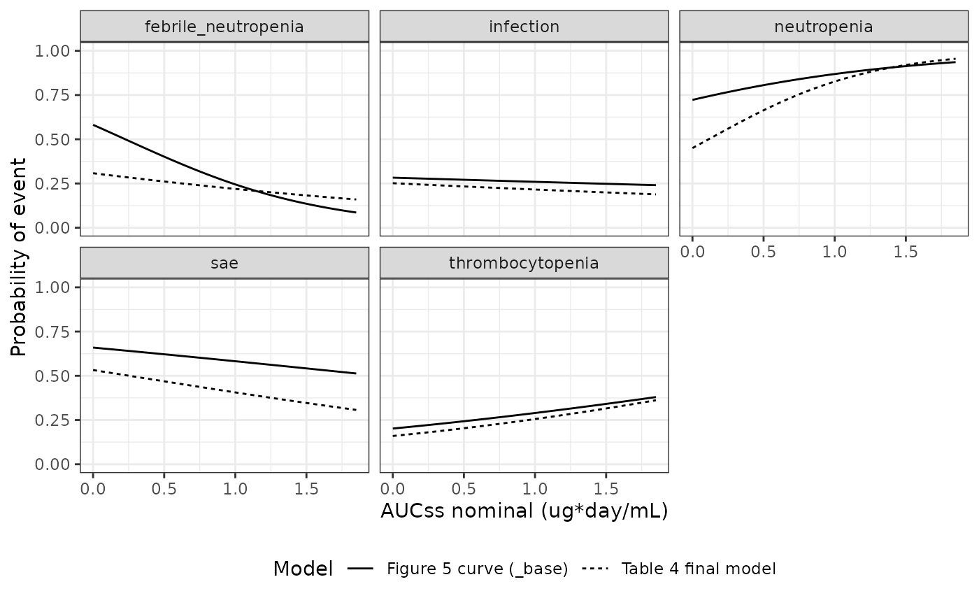
Replicates the fitted curves of Figure 5 of Samineni 2022 (solid, the packaged _base models) alongside the Table 4 final models (dashed) evaluated at a 64-year-old with IPI < 4 and ECOG < 2.
PET-CT complete response (replicates Figure 4)
Figure 4 prints no coefficients, so each fitted line was digitised. The panel headers print event counts that the digitisation never used, which makes them an independent check. Each curve is averaged over exposures on the paper’s scale and compared with its header fraction.
pet <- dplyr::bind_rows(
  data.frame(AUC = auc_grid, Panel = "a: all-comers", Group = "all-comers",
             p = solve_er("petcr", data.frame(AUC_VENETOCLAX_SS = auc_grid))),
  data.frame(AUC = auc_grid, Panel = "b: BCL-2 FISH", Group = "FISH negative",
             p = solve_er("petcr_bcl2_fish", data.frame(AUC_VENETOCLAX_SS = auc_grid, TUM_BCL2_FISH_POS = 0))),
  data.frame(AUC = auc_grid, Panel = "b: BCL-2 FISH", Group = "FISH positive",
             p = solve_er("petcr_bcl2_fish", data.frame(AUC_VENETOCLAX_SS = auc_grid, TUM_BCL2_FISH_POS = 1))),
  data.frame(AUC = auc_grid, Panel = "c: BCL-2 IHC", Group = "IHC high",
             p = solve_er("petcr_bcl2_ihc", data.frame(AUC_VENETOCLAX_SS = auc_grid, TUM_BCL2_IHC_HIGH = 1))),
  data.frame(AUC = auc_grid, Panel = "c: BCL-2 IHC", Group = "IHC low",
             p = solve_er("petcr_bcl2_ihc", data.frame(AUC_VENETOCLAX_SS = auc_grid, TUM_BCL2_IHC_HIGH = 0)))
)
#> Warning: multi-subject simulation without without 'omega'
#> Warning: multi-subject simulation without without 'omega'
#> Warning: multi-subject simulation without without 'omega'
#> Warning: multi-subject simulation without without 'omega'
#> Warning: multi-subject simulation without without 'omega'
ggplot2::ggplot(pet, ggplot2::aes(AUC, p, colour = Group)) +
  ggplot2::geom_line(linewidth = 1) +
  ggplot2::facet_wrap(~Panel) +
  ggplot2::coord_cartesian(ylim = c(0, 1)) +
  ggplot2::labs(x = "AUCss nominal (ug*day/mL)", y = "Probability of PET-CR") +
  ggplot2::theme_bw() +
  ggplot2::theme(legend.position = "bottom")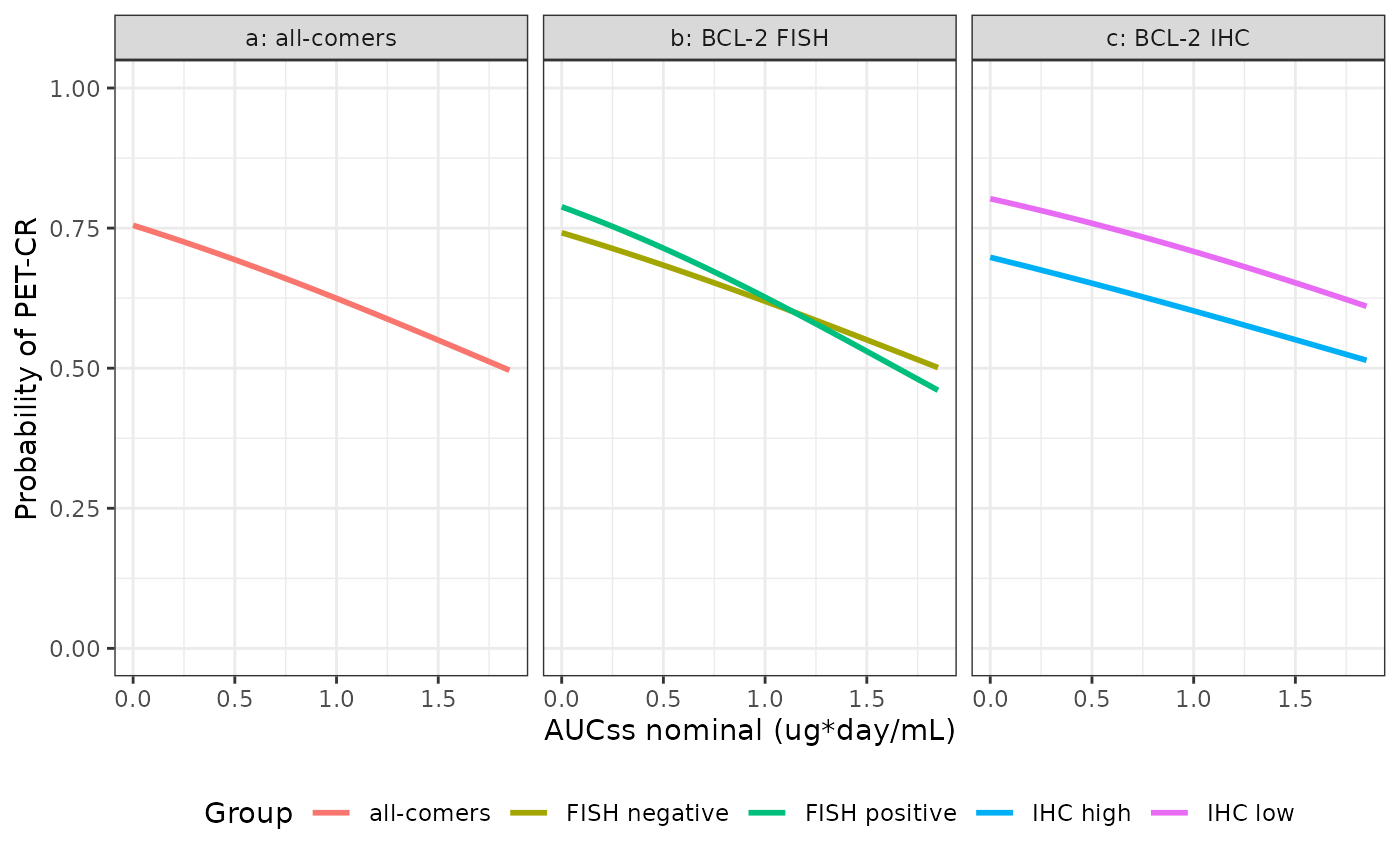
Replicates Figure 4 of Samineni 2022: probability of PET-CT complete response at end of treatment against venetoclax AUCss nominal, for all-comers (a), by BCL-2 FISH (b) and by BCL-2 IHC (c).
auc_paper <- er_cov["AUC_VENETOCLAX_SS"]
pet_check <- tibble::tribble(
  ~Curve,            ~model,             ~ind,                ~val, ~events, ~n,
  "all-comers",      "petcr",            NA_character_,       NA,   136,     199,
  "FISH negative",   "petcr_bcl2_fish",  "TUM_BCL2_FISH_POS", 0,    72,      107,
  "FISH positive",   "petcr_bcl2_fish",  "TUM_BCL2_FISH_POS", 1,    28,      40,
  "IHC high",        "petcr_bcl2_ihc",   "TUM_BCL2_IHC_HIGH", 1,    65,      101,
  "IHC low",         "petcr_bcl2_ihc",   "TUM_BCL2_IHC_HIGH", 0,    54,      72
)
pet_check$predicted <- vapply(seq_len(nrow(pet_check)), function(i) {
  covs <- auc_paper
  if (!is.na(pet_check$ind[i])) covs[[pet_check$ind[i]]] <- pet_check$val[i]
  mean(solve_er(pet_check$model[i], covs))
}, numeric(1))
#> Warning: multi-subject simulation without without 'omega'
#> Warning: multi-subject simulation without without 'omega'
#> Warning: multi-subject simulation without without 'omega'
#> Warning: multi-subject simulation without without 'omega'
#> Warning: multi-subject simulation without without 'omega'
pet_check$observed <- pet_check$events / pet_check$n

stopifnot(all(abs(pet_check$predicted - pet_check$observed) < 0.02))

pet_check |>
  dplyr::transmute(Curve, `Events / patients` = paste0(events, "/", n),
                   `Observed fraction` = round(observed, 3),
                   `Mean predicted` = round(predicted, 3)) |>
knitr::kable(caption = "Digitised PET-CR curves against the event counts printed in the Figure 4 panel headers.")| Curve | Events / patients | Observed fraction | Mean predicted |
|---|---|---|---|
| all-comers | 136/199 | 0.683 | 0.679 |
| FISH negative | 72/107 | 0.673 | 0.670 |
| FISH positive | 28/40 | 0.700 | 0.696 |
| IHC high | 65/101 | 0.644 | 0.641 |
| IHC low | 54/72 | 0.750 | 0.748 |
Every digitised curve reproduces its header fraction to within 0.01. None of the slopes is significant (p = 0.368 all-comers; 0.502 and 0.622 by FISH; 0.622 and 0.704 by IHC), and all are negative. This is the paper’s conclusion: higher venetoclax exposure did not translate into more complete responses at 800 mg.
End-to-end: PK to exposure-response
Chaining the packaged PK model into the exposure-response models
means feeding Eq. 1 exposures into AUC_VENETOCLAX_SS.
Because those exposures run about 1.8 times higher than the paper’s
axis, any model with a non-trivial slope predicts a different event rate
than it does on the paper’s scale. Grade >= 3 neutropenia, the
steepest Table 4 slope, shows it most clearly.
chain <- data.frame(
  Scale = c("Paper exposure axis", "Eq. 1 from the packaged PK model"),
  `Median AUCss (ug*day/mL)` = c(median(er_cov$AUC_VENETOCLAX_SS), median(indiv$auc_eq1)),
  `Mean predicted grade >= 3 neutropenia` = c(
    mean(solve_er("neutropenia", er_cov)),
    mean(solve_er("neutropenia", data.frame(AUC_VENETOCLAX_SS = indiv$auc_eq1)))
  ),
  check.names = FALSE
)
#> Warning: multi-subject simulation without without 'omega'
#> Warning: multi-subject simulation without without 'omega'
knitr::kable(chain, digits = 3, caption = "Grade >= 3 neutropenia on the two exposure scales; observed 149/216 = 0.690.")| Scale | Median AUCss (ug*day/mL) | Mean predicted grade >= 3 neutropenia |
|---|---|---|
| Paper exposure axis | 0.559 | 0.696 |
| Eq. 1 from the packaged PK model | 0.986 | 0.820 |
Assumptions and deviations
-
Legacy parameters encoded as fixed. Samineni 2022
held every legacy value constant and estimated only the two GO27878
study effects, so only those two are free in
ini(). The legacy model itself is Jones et al., AAPS J 2016 (doi:10.1208/s12248-016-9927-9). That paper is not open access, and Table 2 reprints all of its values. -
Low-fat meal is the F1 reference. Table 2 prints
factors for fasting, moderate-fat, high-fat and “fed” meals but none for
low fat, so low fat is taken as the reference (factor 1). The same
lineage states this explicitly (Dave 2019, Table 2 “Low fat on F1” = 1).
CAVALLI’s protocol meals were both classified as low fat (Discussion).
The “fed” level, with the meal type not recorded, is selected by
FED = 1with all three meal indicators 0. - No IIV covariances. Table 2 reports three variances and no covariances, so the three etas are independent. The printed CVs match the square root of the variance: 0.153, 0.205 and 0.097 round to 0.15, 0.21 and 0.10.
-
OATP1B3 inhibitor mapped to
CONMED_OATP1B_INH. The register entry covers OATP1B1 and OATP1B3 jointly. - Rituximab coadministration is not a covariate. The legacy model’s 1.21-fold effect of rituximab on CL/F was dropped in Samineni 2022 (Discussion).
- Exposure scale. Eq. 1 applied to the printed Table 2 gives exposures about 1.8-fold above the paper’s exposure axis (see above). Both the PK model and the exposure-response coefficients are shipped as printed and nothing is tuned. Exposure-response predictions should be made on the paper’s scale. A chained PK-to-response prediction overstates the exposure contribution by that factor.
-
Table 4 against Figure 5. The printed Table 4
coefficients and the drawn Figure 5 lines describe different curves, and
the printed exposure p values go with the drawn lines. Both are
packaged: Table 4 as the final models and the digitised lines as the
_basemodels. - Digitised coefficients. Figure 4 (all three panels) and Figure 5 (all five panels) print no coefficients. The maintainers digitised each fitted line from the 300-dpi figure image: pixel columns along the line were converted with an axis-tick calibration and fitted logit-linear in AUC. An independent second digitisation of Figure 4 agreed to within 0.002 in every coefficient. Colours follow the figure legends (Figure 4b: red negative, blue positive; Figure 4c: red high, blue low), and the header event counts confirm the assignment.
-
IPI reference group. Methods compare IPI 4-5
against IPI 2-3, while the Table 4 footnote says IPI 0, 1 and 2. CAVALLI
enrolled 26 patients with IPI 0-1.
IPI_GE4 = 0is read as every patient with IPI 0 to 3. - Not extracted: progression-free survival. The Cox models of Table 3 report only the exposure coefficient (-0.00181 and -0.2108 per ug*day/mL, p = 0.79 and 0.65) and no baseline hazard, so they cannot be simulated. The relative dose intensity analyses of Figure 6 are correlations, not models.
- Virtual cohort. CYP3A inhibitor, OATP1B3 inhibitor and sex frequencies come from Table 1 and are drawn independently. The exposure-response cohort draws exposures from a log-normal matched to the paper’s quartile bounds, and age, IPI and ECOG independently from Table 1. The paper does not tabulate the 216-patient safety subset, so the 232-patient Table 1 distributions are used.
- Placeholder residual. Each logistic model carries a fixed additive SD of 0.001 on the probability so rxode2 has an error model. It is not a published quantity; the source likelihood is Bernoulli.