Rivipansel (Nayak 2021)

Model and source

Nayak, Tammara and Harnisch (2021) pooled every rivipansel study run before the phase III RESET trial – healthy volunteers, elderly subjects, subjects with renal or hepatic impairment, adults with stable sickle cell disease (SCD) and the phase II study in SCD patients hospitalized for a vaso-occlusive crisis (VOC) – into one population PK analysis. The three-compartment model of Tammara 2017 (Tammara_2017_rivipansel) did not converge on the enlarged dataset, so the authors moved to a two-compartment model and added the urine data from five studies, which splits total clearance into a renal and a non-renal arm.

• Citation: Nayak S, Tammara B, Harnisch LO. Population Pharmacokinetic Analysis of Rivipansel in Healthy Subjects and Subjects with Sickle Cell Disease. Drugs R D. 2021;21(2):217-229.
• Article: https://doi.org/10.1007/s40268-021-00346-3
• The final NONMEM control stream (run58) is published as Electronic Supplementary Material; it fixes every covariate form and reference value used below.

mod <- rxode2::rxode2(readModelDb("Nayak_2021_rivipansel"))
#> ℹ parameter labels from comments will be replaced by 'label()'

Population

The model was fitted to 217 subjects from eight studies (Table 2): 174 phase I subjects and 43 phase II subjects with SCD in VOC. The phase I set was 76% male, 52% White, 36% Black and 8% Asian, aged 19-80 years, and included 28 subjects from the renal-impairment study (7 each with normal, mild, moderate and severe impairment), 16 from the hepatic-impairment study and 14 adults with stable SCD. The phase II set was 58% female and 95% Black, aged 12-56 years, with 13 adolescents aged 12-17 years. Creatinine clearance spans 14.8-214.8 mL/min. The phase III RESET study (156 SCD-VOC patients aged 6 years and older, including 23 children aged 6-11 years) was held out of the fit and used as external validation (Figure 1).

readModelDb("Nayak_2021_rivipansel")$population

Source trace

Equation / parameter	Value	Source location
Two-compartment IV model, ADVAN3 TRANS4, urine as output compartment	–	Methods 2.3, 2.4; ESM control stream $SUBROUTINES, S3 = UVOL
CL = CLR + CLN; urine receives the renal share (F0 = CLR/CL)	–	ESM control stream $PK
CLR = TVCL * exp(eta) * (CRCL/119)^0.477 * (1 + 0.116 * STUDY)	–	Methods 2.3 equations; ESM SCLR, SCLF, MDCRCL3 = 119
Exponent 0.477 + 0.413 when CRCL < 60 mL/min	–	Methods 2.6; ESM IF(CRCL3.LT.60)
Vc, Vp scaled by (WT/75)^0.512	–	Methods 2.3; ESM SWTB, MDWT = 75
Age and weight factors on CLR fixed to exponent 0	–	ESM THETA(8), THETA(11) (0 FIX)
Y = IPRED + sqrt(IPRED^2 + theta^2) * eps (plasma); Y = IPRED * (1 + eps) (urine)	–	Methods 2.3 residual equation; ESM $ERROR
lcl_renal (CL, renal)	1.15 L/h	Table 3
lcl_nonren (CLn)	0.0718 L/h	Table 3
lvc (Vc)	6.75 L	Table 3
lq (Q)	2.01 L/h	Table 3
lvp (Vp)	4.48 L	Table 3
e_study_riv201_cl	0.116	Table 3, fractional increase in CL for SCD-VOC
e_crcl_cl_renal	0.477	Table 3, CrCl factor exponent on CL
e_crcl_cl_renal_lt60	0.413	Table 3, additional exponent at CrCl < 60 mL/min
e_wt_vc_vp	0.512	Table 3, weight factor exponent
IIV CL / Vc / Q / Vp / CLn	20.0 / 32.5 / 24.8 / 22.4 / 82.6 %	Table 3 (square root of variance x 100)
Correlation CL-Vc	0.513	Table 3
Plasma residual: theta SCD-VOC / other	1.53 / 0.865	Table 3, residual error rows
Plasma residual: sqrt(sigma) SCD-VOC / other	21.49 / 9.71 %	Table 3, sigma rows
Urine proportional residual	31.1 %	Table 3

The nlmixr2 combined error is sd = sqrt(propSd^2 * f^2 + addSd^2), which is the control stream’s sqrt(sigma) * sqrt(IPRED^2 + theta^2) with propSd = sqrt(sigma) and addSd = theta * sqrt(sigma):

ini_df <- mod$iniDf
res <- setNames(ini_df$est, ini_df$name)[c(
  "propSd_study201", "addSd_study201", "propSd_nonstudy201", "addSd_nonstudy201"
)]
signif(res, 4)
#>    propSd_study201     addSd_study201 propSd_nonstudy201  addSd_nonstudy201 
#>            0.21490            0.32880            0.09710            0.08399
stopifnot(
  abs(res[["addSd_study201"]] - 1.53 * 0.2149) < 1e-10,
  abs(res[["addSd_nonstudy201"]] - 0.865 * 0.0971) < 1e-10
)

Terminal half-life and renal fraction

Section 2.7 gives the terminal half-life of a two-compartment model and Results report “about 7.5 h” from the Table 3 population estimates. The Discussion reports the renal fraction of total clearance as 0.94.

t_half <- function(cl, vc, q, vp) {
  k10 <- cl / vc
  k12 <- q / vc
  k21 <- q / vp
  s <- k10 + k12 + k21
  log(2) / (0.5 * (s - sqrt(s^2 - 4 * k21 * k10)))
}
tv <- list(clr = 1.15, cln = 0.0718, vc = 6.75, q = 2.01, vp = 4.48)
hl <- tibble::tibble(
  `Clearance used` = c("Renal CL only (1.15 L/h)", "Total CL (1.15 + 0.0718 L/h)"),
  `Terminal t1/2 (h)` = c(
    t_half(tv$clr, tv$vc, tv$q, tv$vp),
    t_half(tv$clr + tv$cln, tv$vc, tv$q, tv$vp)
  )
)
knitr::kable(hl, digits = 2)

Clearance used	Terminal t1/2 (h)
Renal CL only (1.15 L/h)	7.47
Total CL (1.15 + 0.0718 L/h)	7.08

renal_fraction <- tv$clr / (tv$clr + tv$cln)
renal_fraction
#> [1] 0.9412342

stopifnot(
  abs(hl$`Terminal t1/2 (h)`[1] - 7.5) < 0.1,
  abs(renal_fraction - 0.94) < 0.005
)

The paper’s 7.5 h is reproduced with the renal clearance alone; including the non-renal arm shortens the typical terminal half-life to 7.1 h. Both are inside the 7-8 h reported for the phase I studies.

Covariate effects on renal clearance

The renal arm scales with creatinine clearance, with a steeper exponent below 60 mL/min (Section 2.6). As coded, the two branches meet with a step at 60 mL/min rather than joining continuously.

crcl_grid <- tidyr::crossing(CRCL = seq(10, 210, by = 1), STUDY_RIV201 = c(0, 1)) |>
  dplyr::mutate(
    exponent = 0.477 + 0.413 * (CRCL < 60),
    clr = 1.15 * (CRCL / 119)^exponent * (1 + 0.116 * STUDY_RIV201),
    cohort = ifelse(STUDY_RIV201 == 1, "Phase II SCD-VOC", "Other studies")
  )
ggplot(crcl_grid, aes(CRCL, clr, colour = cohort)) +
  geom_line() +
  geom_vline(xintercept = 60, linetype = "dashed", colour = "grey50") +
  labs(x = "Creatinine clearance (mL/min)", y = "Typical renal CL (L/h)", colour = NULL)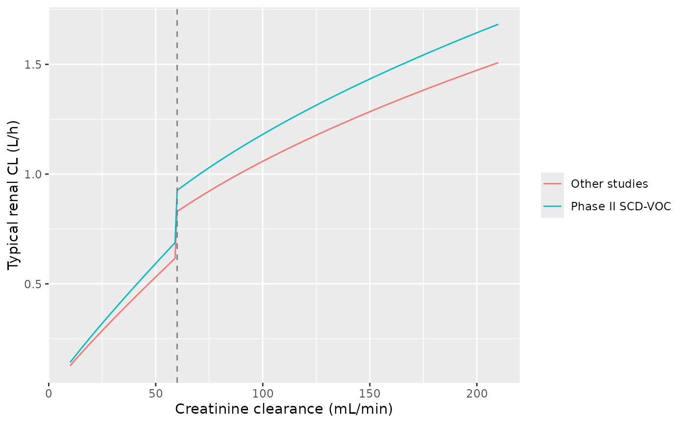

Typical renal clearance against creatinine clearance (non-SCD-VOC and SCD-VOC).

Urinary excretion by renal function

Figure 2 of the paper shows the cumulative percentage of the dose excreted in urine over 96 h in the renal-impairment study (B5201005). The simulation below gives one typical subject (75 kg, not in VOC) per renal-function group; the dose itself cancels out because the model is linear. The creatinine clearance chosen for each group is illustrative. Table 2 reports only the pooled phase I creatinine clearance distribution.

mod_typ <- rxode2::zeroRe(mod)
renal_groups <- tibble::tibble(
  group = factor(
    c("Normal", "Mild", "Moderate", "Severe"),
    levels = c("Normal", "Mild", "Moderate", "Severe")
  ),
  CRCL = c(110, 75, 45, 20)
) |>
  dplyr::mutate(id = dplyr::row_number())

dose_mg <- 1000
inf_dur <- 20 / 60
obs_times <- sort(unique(c(0, seq(0.25, 4, by = 0.25), seq(5, 96, by = 1), 600)))

ev_renal <- dplyr::bind_rows(
  renal_groups |>
    dplyr::mutate(time = 0, amt = dose_mg, rate = dose_mg / inf_dur, evid = 1L, cmt = "central"),
  renal_groups |>
    tidyr::crossing(time = obs_times) |>
    dplyr::mutate(amt = NA_real_, rate = NA_real_, evid = 0L, cmt = NA_character_, dvid = 1L)
) |>
  dplyr::mutate(WT = 75, STUDY_RIV201 = 0, URINE_VOL_INTERVAL = 1000) |>
  dplyr::arrange(id, time, dplyr::desc(evid))

sim_renal <- rxode2::rxSolve(mod_typ, events = ev_renal, returnType = "data.frame", useLinCmt = FALSE,
                             atol = 1e-10, rtol = 1e-10) |>
  dplyr::mutate(id = as.integer(as.character(id))) |>
  dplyr::left_join(dplyr::select(renal_groups, id, group), by = "id") |>
  dplyr::mutate(pct_urine = 100 * urine / dose_mg)
#> ℹ omega/sigma items treated as zero: 'etalcl_renal', 'etalvc', 'etalq', 'etalvp', 'etalcl_nonren'
#> Warning: multi-subject simulation without without 'omega'

ggplot(dplyr::filter(sim_renal, time <= 96), aes(time, pct_urine, colour = group)) +
  geom_line() +
  labs(x = "Time after dose (h)", y = "Cumulative % of dose in urine", colour = "Renal function")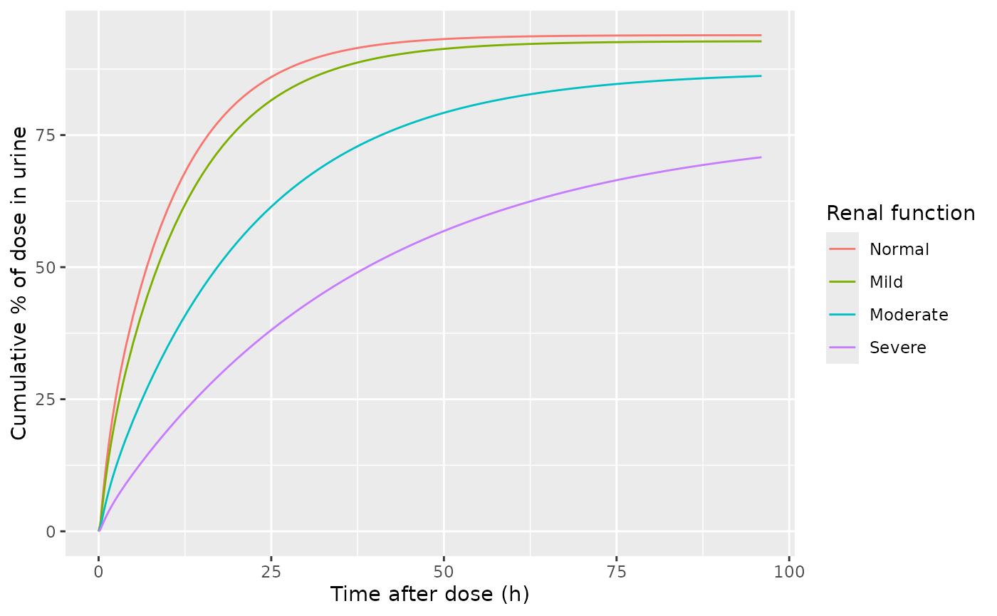

Replicates the model-predicted curves of Figure 2 of Nayak 2021 (typical subjects rather than the study’s individuals). The paper notes the observed normal-renal-function cohort reached only about 77% because of missing data for one subject; the model predicts close to the 94% renal fraction.

at_96 <- sim_renal |> dplyr::filter(time == 96) |> dplyr::select(group, CRCL, pct_urine)
at_inf <- sim_renal |>
  dplyr::filter(time == 600) |>
  dplyr::mutate(
    cl_renal_expected = 1.15 * (CRCL / 119)^(0.477 + 0.413 * (CRCL < 60)),
    fe_expected = 100 * cl_renal_expected / (cl_renal_expected + 0.0718)
  )
dplyr::left_join(at_96, dplyr::select(at_inf, group, pct_inf = pct_urine, fe_expected), by = "group") |>
  dplyr::rename(
    `Renal function` = group,
    `CRCL (mL/min)` = CRCL,
    `% in urine by 96 h` = pct_urine,
    `% in urine at 600 h` = pct_inf,
    `CLR / CL (%)` = fe_expected
  ) |>
  knitr::kable(digits = 1)

Renal function	CRCL (mL/min)	% in urine by 96 h	% in urine at 600 h	CLR / CL (%)
Normal	110	93.9	93.9	93.9
Mild	75	92.7	92.8	92.8
Moderate	45	86.2	87.1	87.1
Severe	20	70.8	76.6	76.6

# Mass balance: once the body is empty the urine holds exactly the renal
# share CLR / (CLR + CLN) of the dose. Same parameters on both sides, so the
# difference is solver error only and a tight bound is correct.
stopifnot(max(abs(at_inf$pct_urine - at_inf$fe_expected)) < 0.01)

Urine concentration per collection interval

A urinary observation is the amount excreted during one collection interval divided by the volume collected (Curine = urine / URINE_VOL_INTERVAL), and the NONMEM stream observes its output compartment with CMT = -3 records, which read the compartment and then empty it. In rxode2 the same reset is a replacement event (evid = 5, amt = 0) on urine, placed a numerical epsilon after each interval boundary so that the end-of-interval observation is taken first.

bounds <- c(4, 8, 12, 24, 48)
vols_ml <- c(400, 350, 300, 900, 1500)
reset_eps <- 1e-6
subj <- tibble::tibble(id = 1L, CRCL = 110, WT = 75, STUDY_RIV201 = 0)

vol_for <- function(t) vols_ml[findInterval(t, c(0, bounds), left.open = TRUE, rightmost.closed = TRUE)]

ev_int <- dplyr::bind_rows(
  subj |> dplyr::mutate(time = 0, amt = dose_mg, rate = dose_mg / inf_dur, evid = 1L, cmt = "central"),
  subj |> tidyr::crossing(time = bounds + reset_eps) |>
    dplyr::mutate(amt = 0, rate = NA_real_, evid = 5L, cmt = "urine"),
  subj |> tidyr::crossing(time = c(0, bounds)) |>
    dplyr::mutate(amt = NA_real_, rate = NA_real_, evid = 0L, cmt = NA_character_, dvid = 1L)
) |>
  dplyr::mutate(URINE_VOL_INTERVAL = ifelse(time == 0, vols_ml[1], vol_for(time))) |>
  dplyr::arrange(id, time, dplyr::desc(evid))

sim_int <- rxode2::rxSolve(mod_typ, events = ev_int, returnType = "data.frame", useLinCmt = FALSE,
                           atol = 1e-10, rtol = 1e-10) |>
  dplyr::filter(time %in% bounds)
#> ℹ omega/sigma items treated as zero: 'etalcl_renal', 'etalvc', 'etalq', 'etalvp', 'etalcl_nonren'
sim_cum <- sim_renal |> dplyr::filter(id == 1, time %in% c(0, bounds))

int_tab <- tibble::tibble(
  `Interval end (h)` = bounds,
  `Urine volume (mL)` = vols_ml,
  `Amount in interval (mg)` = sim_int$urine,
  `Curine (ug/mL)` = sim_int$Curine,
  `Cumulative-run difference (mg)` = diff(sim_cum$urine)
)
knitr::kable(int_tab, digits = 3)

Interval end (h)	Urine volume (mL)	Amount in interval (mg)	Curine (ug/mL)	Cumulative-run difference (mg)
4	400	353.253	883.134	353.253
8	350	187.824	536.640	187.824
12	300	125.807	419.357	125.807
24	900	185.046	205.606	185.046
48	1500	78.249	52.166	78.249

stopifnot(
  max(abs(int_tab$`Amount in interval (mg)` - int_tab$`Cumulative-run difference (mg)`)) < 1e-3,
  max(abs(int_tab$`Curine (ug/mL)` -
            int_tab$`Amount in interval (mg)` / (int_tab$`Urine volume (mL)` / 1000))) < 1e-8
)

Phase II regimens: virtual cohort and steady-state exposure

The phase II study (B5201012) gave a 20 mg/kg loading dose followed by 10 mg/kg every 12 h (low dose) or 40 mg/kg followed by 20 mg/kg every 12 h (high dose). The paper uses the phase II median average steady-state concentrations, 30 and 75 ug/mL, as reference lines in Figures 3-5. The virtual cohort follows the paper’s simulation scheme (Section 2.9): weight and creatinine clearance drawn from normal distributions with the Table 2 mean and CV of the SCD-VOC adults (weight mean 70 kg, CV 22.5%; creatinine clearance mean 144.7 mL/min, CV 19.9%) and adolescents (53 kg, CV 25.7%; 118.7 mL/min, CV 27.6%), in the phase II age mix (70% adults). Table 2 summarises the continuous covariates by age group with the phase II and phase III SCD-VOC patients pooled, so these distributions are those of both studies. Values outside the Table 2 ranges are redrawn. Rivipansel is given as a 20-minute infusion (Tammara 2017).

set.seed(2021)
rxode2::rxSetSeed(2021)
n_per_arm <- 150

draw_trunc <- function(n, mean, cv, lo, hi) {
  out <- numeric(0)
  while (length(out) < n) {
    x <- rnorm(n, mean, mean * cv)
    out <- c(out, x[x >= lo & x <= hi])
  }
  out[seq_len(n)]
}

make_arm <- function(arm, load_mgkg, maint_mgkg, id_offset) {
  n_adult <- round(0.7 * n_per_arm)
  n_ado <- n_per_arm - n_adult
  tibble::tibble(
    id = id_offset + seq_len(n_per_arm),
    treatment = arm,
    age_group = c(rep("Adult", n_adult), rep("12-17 y", n_ado)),
    WT = c(draw_trunc(n_adult, 70, 0.225, 41, 145), draw_trunc(n_ado, 53, 0.257, 31, 81)),
    CRCL = c(draw_trunc(n_adult, 144.7, 0.199, 70.9, 214.8), draw_trunc(n_ado, 118.7, 0.276, 69.4, 203.7)),
    load_mgkg = load_mgkg,
    maint_mgkg = maint_mgkg
  )
}
cohort <- dplyr::bind_rows(
  make_arm("Low dose (20 + 10 mg/kg q12h)", 20, 10, 0L),
  make_arm("High dose (40 + 20 mg/kg q12h)", 40, 20, n_per_arm)
) |>
  dplyr::mutate(STUDY_RIV201 = 1, URINE_VOL_INTERVAL = 1000)

cohort |>
  dplyr::group_by(treatment, age_group) |>
  dplyr::summarise(n = dplyr::n(), `median WT (kg)` = median(WT),
                   `median CRCL (mL/min)` = median(CRCL), .groups = "drop") |>
  knitr::kable(digits = 1)

treatment	age_group	n	median WT (kg)	median CRCL (mL/min)
High dose (40 + 20 mg/kg q12h)	12-17 y	45	54.2	117.9
High dose (40 + 20 mg/kg q12h)	Adult	105	70.8	144.7
Low dose (20 + 10 mg/kg q12h)	12-17 y	45	56.6	105.6
Low dose (20 + 10 mg/kg q12h)	Adult	105	68.1	144.4

tau <- 12
n_maint <- 14
dose_times <- c(0, tau * seq_len(n_maint))
last_start <- max(dose_times)
obs_grid <- sort(unique(c(
  seq(0, last_start, by = 1),
  last_start + c(0, 1 / 6, inf_dur, 0.5, 0.75, 1, 1.5, 2, 3, 4, 6, 8, 10, 12)
)))

dose_rows <- cohort |>
  tidyr::crossing(time = dose_times) |>
  dplyr::mutate(
    amt = ifelse(time == 0, load_mgkg, maint_mgkg) * WT,
    rate = amt / inf_dur, evid = 1L, cmt = "central"
  )
obs_rows <- cohort |>
  tidyr::crossing(time = obs_grid) |>
  dplyr::mutate(amt = NA_real_, rate = NA_real_, evid = 0L, cmt = NA_character_, dvid = 1L)
events <- dplyr::bind_rows(dose_rows, obs_rows) |>
  dplyr::arrange(id, time, dplyr::desc(evid)) |>
  dplyr::select(id, time, amt, rate, evid, cmt, dvid, WT, CRCL, STUDY_RIV201, URINE_VOL_INTERVAL)

sim <- rxode2::rxSolve(mod, events = events, returnType = "data.frame", useLinCmt = FALSE) |>
  dplyr::mutate(id = as.integer(as.character(id))) |>
  dplyr::left_join(dplyr::select(cohort, id, treatment, age_group), by = "id")

sim |>
  dplyr::filter(!is.na(Cc), time > 0) |>
  dplyr::group_by(treatment, time) |>
  dplyr::summarise(
    med = median(Cc), lo = quantile(Cc, 0.05), hi = quantile(Cc, 0.95),
    .groups = "drop"
  ) |>
  ggplot(aes(time, med)) +
  geom_ribbon(aes(ymin = lo, ymax = hi), alpha = 0.25) +
  geom_line() +
  facet_wrap(~treatment) +
  scale_y_log10() +
  labs(x = "Time after first dose (h)", y = "Rivipansel (ug/mL)")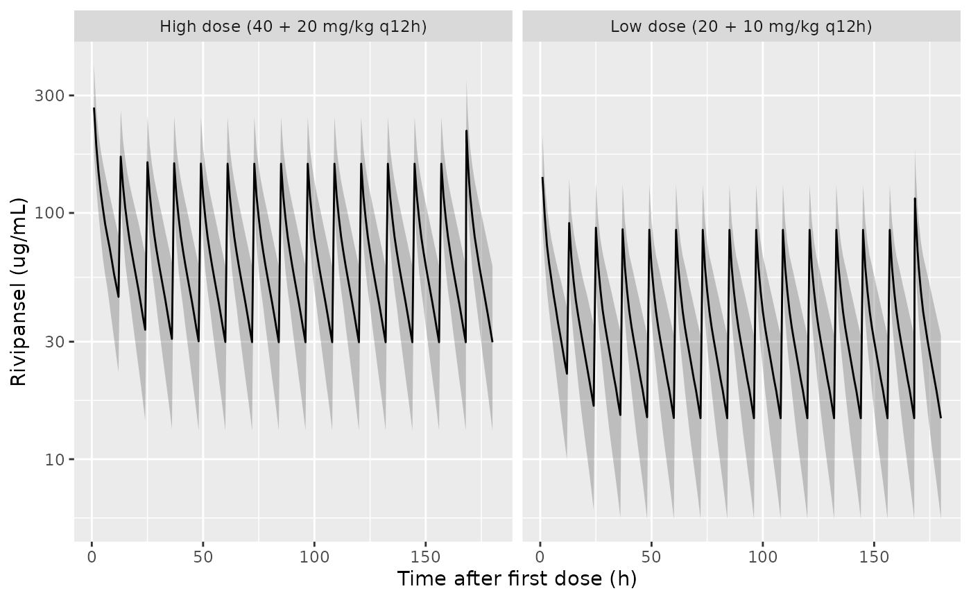

Simulated rivipansel plasma concentrations over 7 days of phase II dosing (median and 90% prediction interval of the individual predictions).

PKNCA over the last dosing interval

conc_ss <- sim |>
  dplyr::filter(time >= last_start, !is.na(Cc)) |>
  dplyr::mutate(tad = time - last_start) |>
  dplyr::select(id, treatment, tad, Cc)
dose_ss <- dose_rows |>
  dplyr::filter(time == last_start) |>
  dplyr::transmute(id, treatment, tad = 0, amt)

conc_obj <- PKNCA::PKNCAconc(conc_ss, Cc ~ tad | treatment + id,
                             concu = "ug/mL", timeu = "h")
dose_obj <- PKNCA::PKNCAdose(dose_ss, amt ~ tad | treatment + id,
                             doseu = "mg", route = "intravascular", duration = inf_dur)
intervals <- data.frame(start = 0, end = tau, cmax = TRUE, cmin = TRUE,
                        auclast = TRUE, cav = TRUE)
nca <- PKNCA::pk.nca(PKNCA::PKNCAdata(conc_obj, dose_obj, intervals = intervals))
nca_df <- as.data.frame(nca$result)

The average steady-state concentration from the NCA must equal the paper’s closed form Cavg,ss = Dose / (CL * tau) (Results), evaluated with each subject’s own total clearance:

cl_ind <- sim |>
  dplyr::filter(time == last_start) |>
  dplyr::distinct(id, cl)
cavg_chk <- nca_df |>
  dplyr::filter(PPTESTCD == "cav") |>
  dplyr::select(id, treatment, cav = PPORRES) |>
  dplyr::left_join(cl_ind, by = "id") |>
  dplyr::left_join(dplyr::select(dose_ss, id, amt), by = "id") |>
  dplyr::mutate(cavg_closed = amt / (cl * tau),
                pct_diff = 100 * (cav - cavg_closed) / cavg_closed)
summary(cavg_chk$pct_diff)
#>    Min. 1st Qu.  Median    Mean 3rd Qu.    Max. 
#> 0.05972 0.14924 0.19253 0.19751 0.24075 0.41574
stopifnot(
  abs(median(cavg_chk$pct_diff)) < 2,
  quantile(abs(cavg_chk$pct_diff), 0.9) < 5
)

The small residual is the remaining approach to steady state of the subjects with the slowest elimination after 7 days, plus trapezoidal error on the infusion peak.

published <- tibble::tribble(
  ~treatment,                          ~cav,
  "Low dose (20 + 10 mg/kg q12h)",     30,
  "High dose (40 + 20 mg/kg q12h)",    75
)
cmp <- nlmixr2lib::ncaComparisonTable(
  simulated = nca,
  reference = published,
  by = "treatment",
  params = "cav",
  units = c(cav = "ug/mL"),
  tolerance_pct = 20
)
knitr::kable(cmp, caption = "Simulated steady-state exposure (median) against the phase II median Cavg,ss quoted in Figures 3-5 of Nayak 2021. * differs from the reference by >20%.")

Simulated steady-state exposure (median) against the phase II median Cavg,ss quoted in Figures 3-5 of Nayak 2021. * differs from the reference by >20%.

NCA parameter	treatment	Reference	Simulated	% diff
Cavg (ug/mL)	Low dose (20 + 10 mg/kg q12h)	30	38.4	+27.9%*
Cavg (ug/mL)	High dose (40 + 20 mg/kg q12h)	75	75.4	+0.5%

The high-dose median matches the paper’s 75 ug/mL. The low-dose median lands above 30 ug/mL: halving the maintenance dose halves the simulated Cavg,ss exactly (the model is linear), whereas the paper’s two phase II medians differ 2.5-fold. The source of the phase II medians (observed or estimated with an earlier model, and on which subjects) is not stated, so the difference is reported rather than adjusted.

Assumptions and deviations

• Model code, not Table 3 labels, sets the covariate structure. The weight exponent is labelled “on Vc” in Table 3 but the control stream (SWTB on V1 and V2) and Methods 2.3 apply it to both volumes. The reference values 75 kg and 119 mL/min exist only in the control stream (MDWT, MDCRCL3); the paper describes them as medians of the fitted data.
• Creatinine clearance is absolute mL/min. The paper says the CKD-EPI (adults) and bedside Schwartz (children) estimates were “normalized by the BSA”. Table 2 shows the direction: children aged 6-11 years with a Schwartz eGFR of about 140 mL/min/1.73 m^2 are tabulated at 91.6 mL/min, so the indexed eGFR was multiplied by BSA / 1.73. Supply CRCL on that scale.
• Age is not a covariate. The Discussion says renal clearance depends on “CrCl, age, and an additional factor”, but the age exponent on renal clearance is (0 FIX) in the final control stream and absent from Table 3. Age acts only through the eGFR equations. The weight exponent on renal clearance is likewise fixed to 0 (Section 2.5).
• SCD-VOC indicator. The clearance increment and the SCD-VOC residual error apply to STUDY.EQ.1012 in the control stream, which is the phase II study NCT01119833 and the same trial as the STUDY_RIV201 indicator of Tammara 2017. Set STUDY_RIV201 = 1 to simulate SCD patients in VOC. The phase III study was not in the fit, and the paper does not say whether its post hoc estimates used the increment.
• Residual-error units and mapping. Table 3 labels the two plasma residual thetas “ng/mL”. Plasma concentrations are in ug/mL (mg doses, L volumes; the paper quotes Cavg,ss and Cmax in ug/mL), and an additive error below 1 ng/mL would be meaningless against concentrations of 10-300 ug/mL, so the thetas are taken in ug/mL. The control-stream comment calls THETA(5) the non-SCD-VOC factor, but $ERROR uses THETA(5) for study
  1012. The mapping here follows the Table 3 labels, which agree with the code (and with the initial estimates 0.355 > 0.113).
• Urine volume units. The control stream divides the urine amount by UVOL without stating its units. URINE_VOL_INTERVAL is taken in mL and converted to L so that Curine is in mg/L (= ug/mL). The urine residual error is purely proportional, so this choice does not affect the fit.
• Infusion duration is not stated in Nayak 2021 (the study-level dosing table referenced as ESM Table 1 is not part of the published supplement, which contains only the control stream). The 20-minute infusion of the rivipansel programme (Tammara 2017) is used.
• Figure 2 renal groups use illustrative creatinine clearances (110, 75, 45, 20 mL/min) because individual values for the renal-impairment study are not reported.
• Not reproduced: the phase III VPC (Figure 1), the phase III post hoc Cavg,ss (Figures 3-5) and the renal-impairment exposure simulation (ESM Table 1). The phase III dosing regimen and its dose adjustments are not given in the paper, and the ESM table is not available.