Linezolid (Gallego-Hernandez 2026)
Source:vignettes/articles/GallegoHernandez_2026_linezolid.Rmd
GallegoHernandez_2026_linezolid.Rmd
library(nlmixr2lib)
library(rxode2)
library(PKNCA)
library(dplyr)
library(ggplot2)

rxode2::rxSetSeed(20260914)
The model
GallegoHernandez_2026_linezolid is a one-compartment
intravenous population PK model for linezolid in elderly hospitalized
patients, built from routine therapeutic-drug-monitoring (TDM) records
at the University Hospital of Salamanca.
mod <- readModelDb("GallegoHernandez_2026_linezolid")
ui <- rxode2::rxode(mod)
#> ℹ parameter labels from comments will be replaced by 'label()'
ui
#>  ── rxode2-based free-form 1-cmt ODE model ──────────────────────────────────────
#>  ── Initalization: ──
#> Fixed Effects ($theta):
#>             lcl             lvc       e_crcl_cl e_tfirstdose_cl        e_age_cl
#>        1.446919        3.242592        0.290000       -0.180000       -1.160000
#>          propSd
#>        0.265000
#>
#> Omega ($omega):
#>          etalcl
#> etalcl 0.110224
#> attr(,"lotriLabels")
#> [1] "Table 2 'IIVCL (CV, %)' = 33.20 -> 0.332^2 (RSE 9%, bootstrap 95% CI 28.3-36.10; eta-shrinkage 4.3%). Base structural model was 42.9% before the three covariates entered."
#> attr(,"lotriFix")
#>        etalcl
#> etalcl  FALSE
#>
#> States ($state or $stateDf):
#>   Compartment Number Compartment Name
#> 1                  1          central
#>  ── μ-referencing ($muRefTable): ──
#>   theta    eta level
#> 1   lcl etalcl    id
#>
#>  ── Model (Normalized Syntax): ──
#> function() {
#>     compartmentData <- list(central = list(analyte = "linezolid",
#>         units = "mg", specimen = "serum", verified = TRUE))
#>     covariateData <- list(CRCL = list(description = "Estimated glomerular filtration rate, CKD-EPI equation, in ABSOLUTE mL/min (de-normalized, NOT mL/min/1.73 m^2).",
#>         units = "mL/min (absolute, NOT BSA-normalized)", type = "continuous",
#>         reference_category = NULL, notes = "Enters clearance as the centred power term (CRCL / 59.56)^0.29 (Results 3.2 final-model equation). Three cautions carry forward. First, the normalisation: Methods 2.1 states that 'the CKD-EPI estimated glomerular filtration rate (eGFR) expressed in absolute values (mL/min) was used', so this column is NOT on the mL/min/1.73 m^2 scale that is this canonical's default, and the paper argues in Discussion that absolute eGFR is the physiologically coherent pairing for a drug clearance. Supplying a BSA-normalized value silently rescales the renal term. Second, the values were CAPPED AT 130 mL/min before fitting, because reduced muscle mass in the elderly depresses serum creatinine and so inflates any creatinine-based estimate (Methods 2.1); a user supplying uncapped data is extrapolating past what was fitted. Third, the column is TIME-VARYING: Methods 2.1 specifies renal function was 'handled as a time-varying covariate, using the value closest to each concentration measurement'. Development-cohort median 48.8 mL/min (IQR 25.9-75.4, Table 1), so the 59.56 centring constant sits ABOVE the cohort median and the typical patient's clearance is below the printed 4.25 L/h. The centring constant appears as 59.56 in the Results 3.2 prose and as the rounded 59.6 inside the printed equation; the two agree to the precision shown and the full-precision form is used here. The paper tested Cockcroft-Gault on several weight descriptors as well and found absolute eGFR the strongest predictor.",
#>         source_name = "eGFR"), AGE = list(description = "Age.",
#>         units = "years", type = "continuous", reference_category = NULL,
#>         notes = "Enters clearance as the centred power term (AGE / 78)^-1.16 (Results 3.2 final-model equation), so clearance FALLS with advancing age. The 78-year centring constant is the development-cohort median (Table 1). Two cautions. First, the exponent is steep (-1.16) but rests on a narrow fitted range of 65-87 years and is the least precisely estimated fixed effect in the model (RSE 43%, bootstrap 95% CI -1.90 to -0.46); across the full observed age range the age multiplier spans only about 1.24 to 0.86, so the steepness is an artefact of extrapolating a power function whose argument barely moves away from 1. It must NOT be extrapolated below 65 years, where it diverges rapidly. Second, age is itself an input to the CKD-EPI equation that produces CRCL, so the two retained covariates are not mechanistically independent; the authors addressed this directly and report only weak collinearity (Spearman rho = -0.203, variance inflation factor 1.05), concluding age carries explanatory information beyond eGFR in this dataset. Treated as time-fixed.",
#>         source_name = "AGE"), T_FIRSTDOSE = list(description = "Time elapsed since the first linezolid dose of the treatment course, i.e. treatment duration.",
#>         units = "h", type = "continuous", reference_category = NULL,
#>         notes = "The paper's DAY covariate, 'treatment duration in days'. Carried in canonical HOURS and divided by 24 inside model() to recover the paper's days, exactly as the T_FIRSTDOSE register entry prescribes and as Eechoute_2012_imatinib.R and Chen_2021_lorlatinib_hypertriglyceridemia.R do. Enters clearance as the centred power term (DAY / 3.5)^-0.18 (Results 3.2 final-model equation), so apparent clearance declines as therapy continues. THIS TERM IS UNDEFINED AT T_FIRSTDOSE = 0: a negative power of zero is infinite, so a simulation must supply a strictly positive value. That is a property of the published model, not an encoding choice, and it is harmless in practice because the fitted data contain no record at day 0 -- the local TDM protocol drew the first sample before the third to fifth dose, giving a median 3 days (IQR 2-4) to the first measurement (Table 1), and treatment duration ran to a median 7 days (range 3-26). The paper's own simulations (Figures 4-6) hold treatment duration FIXED per scenario at 3, 7 and 10 days rather than letting it run as a clock, and the vignette reproduces them that way. Users fitting real TDM records should supply the per-record treatment duration, which makes the column time-varying and monotonically increasing. The authors caution that in a retrospective real-world dataset this covariate may capture concurrent changes in clinical status, inflammation, renal function, TDM-driven dose adaptation or survivor bias as much as any time-dependent pharmacokinetic process (Discussion).",
#>         source_name = "DAY"))
#>     covariatesDataExcluded <- list(WT = list(description = "Total body weight.",
#>         units = "kg", type = "continuous", notes = "Development-cohort median 70 kg (IQR 60-80), Table 1. Screened and not retained. Ideal body weight (median 58.5 kg, IQR 54-64.3), adjusted body weight (0.4 correction factor), body mass index (median 26.6 kg/m^2, IQR 23.8-30.0) and body surface area (Mosteller) were also collected and screened; note that weight descriptors entered the screen chiefly as inputs to alternative Cockcroft-Gault renal-function estimators, all of which lost to absolute CKD-EPI eGFR (Results 3.2)."),
#>         SEXF = list(description = "Female sex indicator.", units = "1 = female, 0 = male",
#>             type = "categorical", notes = "Development cohort 65.0% male, i.e. 35.0% female (Table 1). Screened and not retained."),
#>         ALB = list(description = "Serum albumin.", units = "g/dL",
#>             type = "continuous", notes = "Development-cohort median 3.0 g/dL (IQR 2.7-3.3), Table 1. Screened and not retained."),
#>         CREAT = list(description = "Serum creatinine.", units = "mg/dL",
#>             type = "continuous", notes = "Collected (Methods 2.1) as the input to both the Cockcroft-Gault and CKD-EPI renal-function estimators. Not tabulated as a standalone row in Table 1 and not retained in its raw form; renal function entered the model through CRCL instead."),
#>         ALT = list(description = "Alanine aminotransferase (hepatic-function marker).",
#>             units = "U/L", type = "continuous", notes = "Development-cohort median 24 U/L (IQR 11.5-36.5), Table 1. Screened and not retained."),
#>         AST = list(description = "Aspartate aminotransferase (hepatic-function marker).",
#>             units = "U/L", type = "continuous", notes = "Development-cohort median 44 U/L (IQR 30-77), Table 1. Screened and not retained."),
#>         TBILI = list(description = "Total bilirubin (hepatic-function marker).",
#>             units = "mg/dL", type = "continuous", notes = "Development-cohort median 0.4 mg/dL (IQR 0.3-0.6), Table 1, where it is abbreviated BLT. Screened and not retained."),
#>         LDH = list(description = "Lactate dehydrogenase.", units = "U/L",
#>             type = "continuous", notes = "Development-cohort median 212.0 U/L (IQR 174.5-285.5), Table 1. Screened and not retained."),
#>         TPRO = list(description = "Total serum protein.", units = "g/dL",
#>             type = "continuous", notes = "Development-cohort median 5.5 g/dL (IQR 5.1-6.0), Table 1. Screened and not retained."),
#>         CRP = list(description = "C-reactive protein (inflammation marker).",
#>             units = "mg/L", type = "continuous", notes = "Development-cohort median 9.4 mg/L (IQR 4.0-19.2), Table 1. Screened and not retained."),
#>         PROCALCITONIN = list(description = "Serum procalcitonin (inflammation / sepsis marker).",
#>             units = "ng/mL", type = "continuous", notes = "Development-cohort median 0.5 ng/mL (IQR 0.2-1.3), Table 1. Screened and not retained."),
#>         HGB = list(description = "Haemoglobin.", units = "g/dL",
#>             type = "continuous", notes = "Development-cohort median 10.1 g/dL (IQR 9.0-11.6), Table 1. Collected as a linezolid haematological-toxicity marker as well as a screened covariate. Not retained."),
#>         PLT = list(description = "Platelet count.", units = "10^9/L",
#>             type = "continuous", notes = "Development-cohort median 241 x10^9/L (IQR 172.5-349.5), Table 1. Collected chiefly as the linezolid thrombocytopenia marker. Not retained."),
#>         CONMED_RIF = list(description = "Concomitant rifampicin indicator (a known inducer).",
#>             units = "1 = yes, 0 = no", type = "categorical",
#>             notes = "3 of 103 development-cohort patients (2.9%), Table 1. Methods 2.1 states that concomitant medications with potential pharmacokinetic interaction were recorded 'with particular attention to known enzyme or transporter inducers and inhibitors, including rifampicin and macrolides'. Not retained; at n = 3 the cohort carries almost no information about this interaction."),
#>         CONMED_MACROLIDE = list(description = "Concomitant macrolide indicator.",
#>             units = "1 = yes, 0 = no", type = "categorical",
#>             notes = "7 of 103 development-cohort patients (6.8%), Table 1. Screened per Methods 2.1 and not retained."),
#>         CONMED_PPI = list(description = "Concomitant proton-pump-inhibitor indicator.",
#>             units = "1 = yes, 0 = no", type = "categorical",
#>             notes = "88 of 103 development-cohort patients (85.4%), Table 1. Recorded as part of the polypharmacy profile; not retained. Note the near-universal prevalence leaves little contrast to estimate an effect from."),
#>         CONMED_AZOLE = list(description = "Concomitant azole antifungal indicator (CYP3A4 / P-gp inhibitor).",
#>             units = "1 = yes, 0 = no", type = "categorical",
#>             notes = "13 of 103 development-cohort patients (12.6%), Table 1. Screened per Methods 2.1 and not retained."))
#>     description <- "One-compartment intravenous population PK model for linezolid in elderly hospitalized patients aged 65-87 years (Gallego-Hernandez 2026), developed from routine therapeutic-drug-monitoring records at a single Spanish tertiary hospital. Clearance (4.25 L/h typical) carries three centred power covariates: absolute CKD-EPI eGFR (exponent 0.29, referenced to the population median 59.56 mL/min), treatment duration in days (exponent -0.18, referenced to 3.5 days) and age (exponent -1.16, referenced to 78 years). The treatment-duration term is the paper's novel finding: apparent clearance declines progressively over a course of therapy, which the authors describe as a phenomenological description of the observed data rather than evidence of a specific biological mechanism. Central volume is a single typical value of 25.6 L with no covariates and no interindividual variability, the predominantly trough-oriented sampling design having been unable to support either. Interindividual variability is carried on clearance alone (33.2% CV) and residual error is proportional (26.5% CV). The model is intended as a Bayesian TDM tool for detecting linezolid overexposure in the elderly, not as a fully descriptive structural model."
#>     population <- list(species = "human", n_subjects = 103, n_studies = 1,
#>         age_median = "78 years (range 65-87)", age_range = "65-87 years",
#>         weight_median = "70 kg (IQR 60-80)", bmi_median = "26.6 kg/m^2 (IQR 23.8-30.0)",
#>         sex_female_pct = 35, race_ethnicity = "Single-centre Spanish cohort; race/ethnicity not reported in the source.",
#>         disease_state = "Elderly hospitalized adults receiving intravenous linezolid as targeted or empirical therapy for Gram-positive infection. Diagnoses in the development cohort were respiratory infection 21.4%, skin and soft tissue infection 22.3%, urinary tract infection 23.3% and other infections 33.0% (Table 1). Patients on oral linezolid, with active oncological or haematological disease, on renal replacement therapy, or critically ill requiring ICU admission were EXCLUDED by design, so the model carries no information about those groups.",
#>         renal_function = "Broad and skewed towards impairment: absolute CKD-EPI eGFR median 48.8 mL/min (IQR 25.9-75.4). Strata: >90 mL/min 11.7%, 60-89 mL/min 26.2%, 30-59 mL/min 32.0%, <30 mL/min 30.1% (Table 1). Values were capped at 130 mL/min for modelling. Renal replacement therapy was an exclusion criterion.",
#>         dose_range = "All patients started intravenous linezolid 600 mg every 12 h as a 1-h infusion, after which dosing was individualized on TDM results. Development-cohort daily dose median 1200 mg/day (range 300-1800), maximum daily dose median 1200 mg/day (range 600-2400), daily dose per body weight median 14.7 mg/kg/day (IQR 10.0-17.7). Treatment duration median 7 days (range 3-26).",
#>         regions = "Spain (University Hospital of Salamanca).",
#>         notes = "Retrospective, single-centre study of routine TDM records, January 2024 to September 2025. 149 patients contributing 293 quantifiable serum concentrations were randomly split about 2:1 into a development cohort of 103 patients / 198 concentrations (the fit this model reproduces) and an independent validation cohort of 46 patients / 95 concentrations. A further 15 measurements below the 0.8 mg/L assay LLOQ were excluded rather than handled by an M-method. Sampling is predominantly TROUGH-ORIENTED and sparse -- median 2 samples per patient (range 1-5), the first drawn before the third to fifth dose -- which is the stated reason the model carries no peripheral compartment and no IIV on volume, and why the authors call it a pragmatic TDM tool rather than a fully descriptive structural model. Concentrations were measured by ENZYME IMMUNOASSAY (ARK Linezolid Assay on an Abbott Architect ci4100), not LC-MS/MS, with limited reported cross-reactivity against the inactive linezolid metabolites; the authors flag this as a contributor to residual variability. Independent-validation performance was a mean prediction error of -10.54% and a mean absolute prediction error of 47.8%, which the authors contextualise against an external evaluation in which 25 published linezolid models returned median MAPEs of 58-73%. Estimation was FOCE-I in NONMEM 7.5 with PsN 5.3.1; the final model was confirmed by a 1000-replicate bootstrap (990 successful). Development-cohort mean observed concentration 6.5 mg/L (SD 4.0).")
#>     reference <- "Gallego-Hernandez G, Albarran-Gomez A, Sanchez-Hernandez JG, Garcia-Casanueva JC, Otero MJ. Population Pharmacokinetics of Linezolid in Elderly Hospitalized Patients: Implications for Therapeutic Drug Monitoring. Pharmaceutics. 2026;18(5):528. doi:10.3390/pharmaceutics18050528"
#>     units <- list(time = "h", dosing = "mg", concentration = "mg/L")
#>     vignette <- "GallegoHernandez_2026_linezolid"
#>     ini({
#>         lcl <- 1.44691898293633
#>         label("Clearance at the reference covariate values (L/h)")
#>         lvc <- 3.24259235148552
#>         label("Central volume of distribution, V (L)")
#>         e_crcl_cl <- 0.29
#>         label("Power exponent for absolute CKD-EPI eGFR on CL (unitless)")
#>         e_tfirstdose_cl <- -0.18
#>         label("Power exponent for treatment duration on CL (unitless)")
#>         e_age_cl <- -1.16
#>         label("Power exponent for age on CL (unitless)")
#>         propSd <- c(0, 0.265)
#>         label("Proportional residual SD for Cc (fraction)")
#>         etalcl ~ 0.110224
#>         label("Table 2 'IIVCL (CV, %)' = 33.20 -> 0.332^2 (RSE 9%, bootstrap 95% CI 28.3-36.10; eta-shrinkage 4.3%). Base structural model was 42.9% before the three covariates entered.")
#>     })
#>     model({
#>         crcl_ref <- 59.56
#>         day_ref <- 3.5
#>         age_ref <- 78
#>         day_trt <- T_FIRSTDOSE/24
#>         cl <- exp(lcl + etalcl) * (CRCL/crcl_ref)^e_crcl_cl *
#>             (day_trt/day_ref)^e_tfirstdose_cl * (AGE/age_ref)^e_age_cl
#>         vc <- exp(lvc)
#>         kel <- cl/vc
#>         d/dt(central) <- -kel * central
#>         Cc <- central/vc
#>         Cc ~ prop(propSd)
#>     })
#> }
Clearance carries three centred power covariates. The final-model equation is printed in the paper’s Results section 3.2:
The DAY term is the paper’s novel contribution: apparent
clearance falls progressively over a course of therapy. The authors are
explicit that this is “a phenomenological description of the observed
data rather than … direct evidence of a specific biological mechanism” –
in a retrospective real-world dataset it may also absorb concurrent
changes in clinical status, inflammation, renal function, TDM-driven
dose adaptation, or survivor bias.
Central volume is a single typical value of 25.6 L. Neither a peripheral compartment (dOFV only about 11.7, and the peripheral volume had RSE 69%) nor interindividual variability on volume was supported by the predominantly trough-oriented sampling design.
Population
pop <- ui$population
tibble::tibble(Field = names(pop), Value = vapply(pop, paste, character(1), collapse = "; ")) |>
knitr::kable(caption = "Population metadata recorded with the model.")| Field | Value |
|---|---|
| species | human |
| n_subjects | 103 |
| n_studies | 1 |
| age_median | 78 years (range 65-87) |
| age_range | 65-87 years |
| weight_median | 70 kg (IQR 60-80) |
| bmi_median | 26.6 kg/m^2 (IQR 23.8-30.0) |
| sex_female_pct | 35 |
| race_ethnicity | Single-centre Spanish cohort; race/ethnicity not reported in the source. |
| disease_state | Elderly hospitalized adults receiving intravenous linezolid as targeted or empirical therapy for Gram-positive infection. Diagnoses in the development cohort were respiratory infection 21.4%, skin and soft tissue infection 22.3%, urinary tract infection 23.3% and other infections 33.0% (Table 1). Patients on oral linezolid, with active oncological or haematological disease, on renal replacement therapy, or critically ill requiring ICU admission were EXCLUDED by design, so the model carries no information about those groups. |
| renal_function | Broad and skewed towards impairment: absolute CKD-EPI eGFR median 48.8 mL/min (IQR 25.9-75.4). Strata: >90 mL/min 11.7%, 60-89 mL/min 26.2%, 30-59 mL/min 32.0%, <30 mL/min 30.1% (Table 1). Values were capped at 130 mL/min for modelling. Renal replacement therapy was an exclusion criterion. |
| dose_range | All patients started intravenous linezolid 600 mg every 12 h as a 1-h infusion, after which dosing was individualized on TDM results. Development-cohort daily dose median 1200 mg/day (range 300-1800), maximum daily dose median 1200 mg/day (range 600-2400), daily dose per body weight median 14.7 mg/kg/day (IQR 10.0-17.7). Treatment duration median 7 days (range 3-26). |
| regions | Spain (University Hospital of Salamanca). |
| notes | Retrospective, single-centre study of routine TDM records, January 2024 to September 2025. 149 patients contributing 293 quantifiable serum concentrations were randomly split about 2:1 into a development cohort of 103 patients / 198 concentrations (the fit this model reproduces) and an independent validation cohort of 46 patients / 95 concentrations. A further 15 measurements below the 0.8 mg/L assay LLOQ were excluded rather than handled by an M-method. Sampling is predominantly TROUGH-ORIENTED and sparse – median 2 samples per patient (range 1-5), the first drawn before the third to fifth dose – which is the stated reason the model carries no peripheral compartment and no IIV on volume, and why the authors call it a pragmatic TDM tool rather than a fully descriptive structural model. Concentrations were measured by ENZYME IMMUNOASSAY (ARK Linezolid Assay on an Abbott Architect ci4100), not LC-MS/MS, with limited reported cross-reactivity against the inactive linezolid metabolites; the authors flag this as a contributor to residual variability. Independent-validation performance was a mean prediction error of -10.54% and a mean absolute prediction error of 47.8%, which the authors contextualise against an external evaluation in which 25 published linezolid models returned median MAPEs of 58-73%. Estimation was FOCE-I in NONMEM 7.5 with PsN 5.3.1; the final model was confirmed by a 1000-replicate bootstrap (990 successful). Development-cohort mean observed concentration 6.5 mg/L (SD 4.0). |
The development cohort is 103 patients contributing 198 quantifiable serum concentrations, drawn from 149 patients / 293 concentrations by a roughly 2:1 random split; the remaining 46 patients / 95 concentrations formed an independent validation cohort. Renal function is broad and skewed towards impairment (absolute CKD-EPI eGFR median 48.8 mL/min, IQR 25.9-75.4, with 30.1% of the cohort below 30 mL/min), which is what gives the model its leverage on the renal term. Patients on renal replacement therapy, on oral linezolid, with active oncological or haematological disease, or critically ill in the ICU were excluded by design.
Source trace
Every value in ini() and every constant in
model() traces to the following locations in
Gallego-Hernandez 2026.
| Quantity | Value | Source location |
|---|---|---|
| Structural model | 1 compartment, first-order elimination, IV | Results 3.2; Abstract |
| CLpop | 4.25 L/h (RSE 9%) | Table 2, row ‘CLpop (L/h)’ |
| Vpop | 25.60 L (RSE 17%) | Table 2, row ‘Vpop (L)’ |
| eGFR exponent on CL | 0.29 (RSE 16%) | Table 2, row ‘eGFR-CL’; Results 3.2 equation |
| Treatment-duration exponent on CL | -0.18 (RSE 14%) | Table 2, row ‘DAY-CL’; Results 3.2 equation |
| Age exponent on CL | -1.16 (RSE 43%) | Table 2, row ‘AGE-CL’; Results 3.2 equation |
| eGFR centring constant | 59.56 mL/min | Results 3.2 prose (‘population median value of 59.56 mL/min’); equation prints rounded 59.6 |
| Treatment-duration centring constant | 3.5 days | Results 3.2 prose and equation |
| Age centring constant | 78 years | Results 3.2 prose and equation; Table 1 median age |
| IIV on CL | 33.20% CV -> omega^2 = 0.110224 | Table 2, row ‘IIVCL (CV, %)’ |
| IIV on V | not estimated (excluded) | Results 3.2 |
| Residual error | proportional, 26.50% CV -> propSd 0.265 | Table 2, row ‘RUVprop (CV, %)’; Results 3.2 |
| Dosing regimen simulated | 600 mg IV q12h, 1-h infusion | Methods 2.5; Results 3.4 |
| Simulation scenarios | eGFR 25/45/75 mL/min; days 3/7/10; age 78 | Results 3.4 and Figure 4 caption |
Structural checks
Before simulating a cohort, confirm the encoded clearance equation reproduces the published one exactly, and that the solved model conserves mass.
published_cl <- function(egfr, day, age = 78) {
  4.25 * (egfr / 59.56)^0.29 * (day / 3.5)^-0.18 * (age / 78)^-1.16
}

scenarios <- tidyr::expand_grid(
  day  = c(3, 7, 10),
  egfr = c(25, 45, 75)
) |>
  mutate(
    scenario = sprintf("Day %d, eGFR %d mL/min", day, egfr),
    cl_published = published_cl(egfr, day)
  )

knitr::kable(
  scenarios |> select(scenario, `CL (L/h)` = cl_published),
  digits = 3,
  caption = "Typical clearance per simulated scenario, from the published equation."
)| scenario | CL (L/h) |
|---|---|
| Day 3, eGFR 25 mL/min | 3.397 |
| Day 3, eGFR 45 mL/min | 4.028 |
| Day 3, eGFR 75 mL/min | 4.672 |
| Day 7, eGFR 25 mL/min | 2.917 |
| Day 7, eGFR 45 mL/min | 3.459 |
| Day 7, eGFR 75 mL/min | 4.011 |
| Day 10, eGFR 25 mL/min | 2.735 |
| Day 10, eGFR 45 mL/min | 3.244 |
| Day 10, eGFR 75 mL/min | 3.761 |
Now solve the model with the random effects zeroed and confirm the
cl it returns equals the closed form. This is a
deterministic comparison of two routes to the same number, so it is
asserted tightly.
tau <- 12          # dosing interval, h
n_dose <- 14       # doses to reach steady state (t_half <= 6.5 h, so ample)
t_last <- tau * (n_dose - 1)
# length.out (not by =) so both interval ends land on EXACTLY t_last and
# t_last + tau: the steady-state check below selects those two times by
# equality, and auclast needs the interval to be fully spanned.
obs_times <- t_last + seq(0, tau, length.out = 121)

build_events <- function(egfr, day, ids) {
  dose <- data.frame(
    id = ids, time = 0, amt = 600, rate = 600, evid = 1L,
    cmt = "central", ii = tau, addl = n_dose - 1L
  )
  obs <- expand.grid(id = ids, time = obs_times, KEEP.OUT.ATTRS = FALSE)
  obs <- transform(
    obs,
    amt = NA_real_, rate = NA_real_, evid = 0L,
    cmt = "central", ii = 0, addl = 0L
  )
  ev <- rbind(dose, obs[names(dose)])
  ev$CRCL <- egfr
  ev$AGE <- 78
  ev$T_FIRSTDOSE <- day * 24          # canonical hours; model divides by 24
  ev$scenario <- sprintf("Day %d, eGFR %d mL/min", day, egfr)
  ev[order(ev$id, ev$time, -ev$evid), ]
}

ev_typ <- do.call(
  rbind,
  Map(
    function(g, d, i) build_events(g, d, i),
    scenarios$egfr, scenarios$day, seq_len(nrow(scenarios))
  )
)

sim_typ <- rxode2::rxSolve(
  rxode2::zeroRe(mod), ev_typ,
  keep = c("scenario", "CRCL", "T_FIRSTDOSE")
) |>
  as.data.frame()
#> ℹ parameter labels from comments will be replaced by 'label()'
#> ℹ omega/sigma items treated as zero: 'etalcl'
#> Warning: multi-subject simulation without without 'omega'

cl_check <- sim_typ |>
  group_by(scenario) |>
  summarise(cl_model = mean(cl), vc_model = mean(vc), .groups = "drop") |>
  left_join(scenarios |> select(scenario, cl_published), by = "scenario") |>
  mutate(rel_diff = abs(cl_model - cl_published) / cl_published)

stopifnot(
  # Deterministic: the model's cl and the published equation are two routes to
  # one number, so any difference is floating point only.
  max(cl_check$rel_diff) < 1e-10,
  # Volume carries no covariates and no IIV.
  all(abs(cl_check$vc_model - 25.6) < 1e-10)
)

knitr::kable(
  cl_check |> select(scenario, cl_published, cl_model, rel_diff),
  digits = c(0, 4, 4, 12),
  caption = "Encoded clearance matches the published equation exactly."
)| scenario | cl_published | cl_model | rel_diff |
|---|---|---|---|
| Day 10, eGFR 25 mL/min | 2.7352 | 2.7352 | 0 |
| Day 10, eGFR 45 mL/min | 3.2435 | 3.2435 | 0 |
| Day 10, eGFR 75 mL/min | 3.7614 | 3.7614 | 0 |
| Day 3, eGFR 25 mL/min | 3.3971 | 3.3971 | 0 |
| Day 3, eGFR 45 mL/min | 4.0284 | 4.0284 | 0 |
| Day 3, eGFR 75 mL/min | 4.6716 | 4.6716 | 0 |
| Day 7, eGFR 25 mL/min | 2.9165 | 2.9165 | 0 |
| Day 7, eGFR 45 mL/min | 3.4586 | 3.4586 | 0 |
| Day 7, eGFR 75 mL/min | 4.0108 | 4.0108 | 0 |
Replicating Figure 4: concentration-time profiles by renal function and treatment day
The paper’s Figure 4 simulates 600 mg IV every 12 h (1-h infusion) across three absolute eGFR values (25, 45, 75 mL/min – the cohort’s 25th, 50th and 75th percentiles) and three treatment durations (3, 7, 10 days), with age fixed at the population median of 78 years.
Treatment duration is held fixed per scenario rather than allowed to run as a clock, which is exactly what the paper does: each panel is a steady-state profile evaluated at that day’s clearance. See the Assumptions section.
n_per_arm <- 150   # paper used 1000 per scenario; 150 is ample for these medians

ev_cohort <- do.call(
  rbind,
  Map(
    function(g, d, k) build_events(g, d, (k - 1) * n_per_arm + seq_len(n_per_arm)),
    scenarios$egfr, scenarios$day, seq_len(nrow(scenarios))
  )
)

sim <- rxode2::rxSolve(
  mod, ev_cohort,
  keep = c("scenario", "CRCL", "T_FIRSTDOSE")
) |>
  as.data.frame() |>
  mutate(
    tad = time - t_last,
    day = as.integer(round(T_FIRSTDOSE / 24)),
    egfr = CRCL
  )
#> ℹ parameter labels from comments will be replaced by 'label()'

stopifnot(
  nrow(sim) > 0,
  !anyNA(sim$Cc),
  all(sim$Cc >= 0),
  dplyr::n_distinct(sim$id) == n_per_arm * nrow(scenarios)
)
profile <- sim |>
  group_by(day, egfr, tad) |>
  summarise(
    med = median(Cc),
    lo = quantile(Cc, 0.05),
    hi = quantile(Cc, 0.95),
    .groups = "drop"
  )

ggplot(profile, aes(tad, med)) +
  annotate("rect", xmin = -Inf, xmax = Inf, ymin = 2, ymax = 7, alpha = 0.15) +
  geom_hline(yintercept = c(2, 7), linetype = "dashed", linewidth = 0.3) +
  geom_ribbon(aes(ymin = lo, ymax = hi), alpha = 0.25, fill = "steelblue") +
  geom_line(colour = "steelblue", linewidth = 0.7) +
  facet_grid(
    rows = vars(paste0("eGFR ", egfr, " mL/min")),
    cols = vars(paste0("Day ", day))
  ) +
  labs(
    x = "Time since last dose (h)",
    y = "Linezolid concentration (mg/L)"
  ) +
  theme_bw()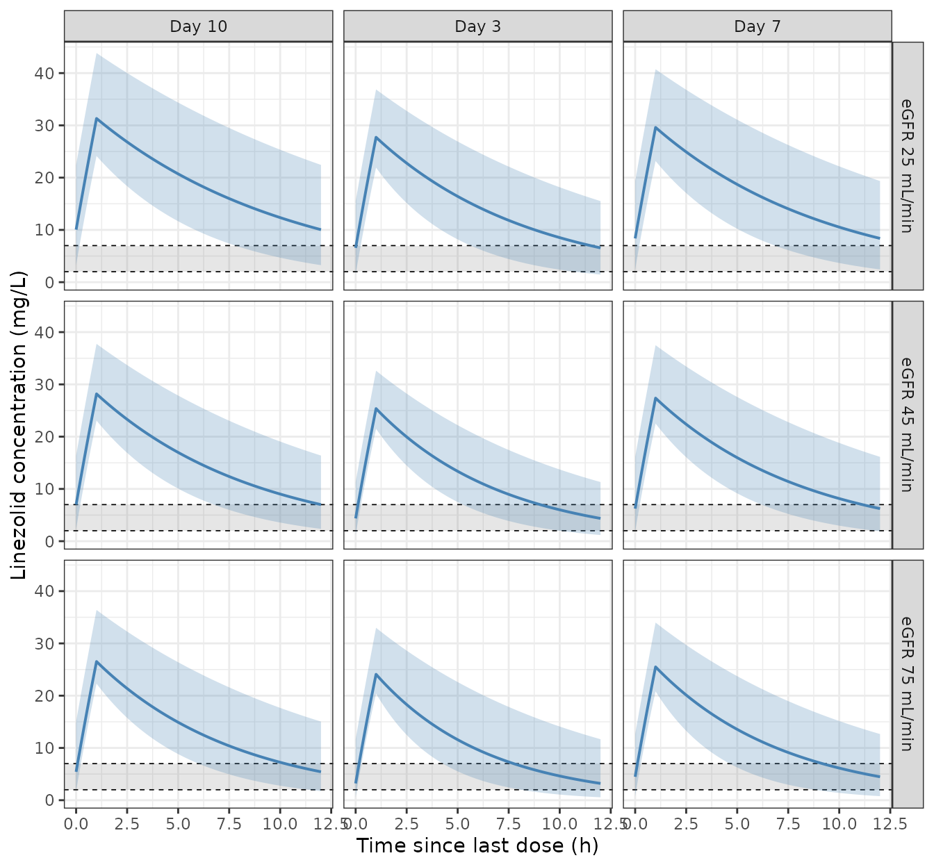
Replicates Figure 4 of Gallego-Hernandez 2026: steady-state linezolid concentration-time profiles under 600 mg IV every 12 h across renal function and treatment duration. Solid line is the median, ribbon the 5th-95th percentile. The grey band is the 2-7 mg/L therapeutic trough range.
PKNCA validation
Steady-state NCA over the final dosing interval. The interval start coincides with an observation record, so no time-zero back-extrapolation is needed.
sim_nca <- sim |>
  dplyr::filter(!is.na(Cc)) |>
  dplyr::select(id, time, Cc, scenario)

dose_nca <- ev_cohort |>
  dplyr::filter(evid == 1) |>
  dplyr::select(id, scenario) |>
  dplyr::distinct() |>
  tidyr::expand_grid(time = seq(0, t_last, by = tau)) |>
  dplyr::mutate(amt = 600) |>
  dplyr::select(id, time, amt, scenario)

conc_obj <- PKNCA::PKNCAconc(
  sim_nca, Cc ~ time | scenario + id,
  concu = "mg/L", timeu = "h"
)
dose_obj <- PKNCA::PKNCAdose(
  dose_nca, amt ~ time | scenario + id,
  doseu = "mg"
)

intervals <- data.frame(
  start = t_last,
  end = t_last + tau,
  cmax = TRUE,
  tmax = TRUE,
  cmin = TRUE,
  cav = TRUE,
  auclast = TRUE
)

nca_res <- PKNCA::pk.nca(
  PKNCA::PKNCAdata(conc_obj, dose_obj, intervals = intervals)
)

nca <- as.data.frame(nca_res$result) |>
  dplyr::select(scenario, id, PPTESTCD, PPORRES) |>
  tidyr::pivot_wider(names_from = PPTESTCD, values_from = PPORRES)

stopifnot(
  nrow(nca) == n_per_arm * nrow(scenarios),
  !anyNA(nca$auclast),
  !anyNA(nca$cmin)
)
cmin rather than ctrough is used as the
steady-state trough below. PKNCA normalizes concentration times to
time after the most recent dose but passes the interval
end through as an absolute time, so
pk.calc.ctrough()’s time %in% end test can
never match and ctrough returns NA for every
subject.
Over this interval the concentration rises during the 1-h infusion
and then declines monotonically, so the interval minimum is attained at
one of its two endpoints. Accumulation approaches steady state from
below, which makes the minimum the trough at the interval’s
start rather than its end. The next check confirms the two
endpoints agree to within a negligible margin, so cmin is
the steady-state trough for practical purposes – and where it differs it
errs low, which is the conservative direction for the overexposure
claims below.
trough_gap <- function(df) {
  df |>
    dplyr::filter(time %in% c(t_last, t_last + tau)) |>
    dplyr::select(id, scenario, time, Cc) |>
    tidyr::pivot_wider(names_from = time, values_from = Cc, names_prefix = "t") |>
    dplyr::mutate(
      rel_diff = abs(.data[[paste0("t", t_last + tau)]] - .data[[paste0("t", t_last)]]) /
        .data[[paste0("t", t_last)]]
    )
}

# Gate on the TYPICAL-VALUE solve. This is fully deterministic -- one subject
# per scenario with the random effects zeroed -- so the bound is reproducible
# on any machine and at any thread count.
ss_typ <- trough_gap(sim_typ)

stopifnot(
  nrow(ss_typ) == nrow(scenarios),
  max(ss_typ$rel_diff) < 1e-5
)

# The cohort equivalent is REPORTED, not gated. Its maximum is the single
# slowest-clearing draw and it enters as exp(-k * t_last), so it swings by
# orders of magnitude with the cohort -- and rxSetSeed() fixes the draw per
# thread count, not across them. Gating it would be a CI-only failure waiting
# to happen.
ss_cohort <- trough_gap(sim)

cat(sprintf(
  paste0(
    "Steady state, typical values: max relative trough gap = %.2e (gated < 1e-5)\n",
    "Steady state, full cohort:    max relative trough gap = %.2e (reported only)\n"
  ),
  max(ss_typ$rel_diff), max(ss_cohort$rel_diff)
))
#> Steady state, typical values: max relative trough gap = 4.20e-08 (gated < 1e-5)
#> Steady state, full cohort:    max relative trough gap = 6.38e-04 (reported only)
Finally, assert rather than merely assert in prose that the interval
minimum is attained at an endpoint. An interior minimum would mean
cmin is not the trough at all, and it would be wrong by
orders of magnitude rather than by a solver tolerance – so this check
can genuinely go red.
endpoint_min <- sim |>
  dplyr::filter(time %in% c(t_last, t_last + tau)) |>
  dplyr::group_by(scenario, id) |>
  dplyr::summarise(endpoint_min = min(Cc), .groups = "drop")

cmin_check <- nca |>
  dplyr::select(scenario, id, cmin) |>
  dplyr::left_join(endpoint_min, by = c("scenario", "id")) |>
  dplyr::mutate(rel_diff = abs(cmin - endpoint_min) / endpoint_min)

stopifnot(
  nrow(cmin_check) == n_per_arm * nrow(scenarios),
  !anyNA(cmin_check$rel_diff),
  # Relative, not absolute: the terminal decline is flat enough that solver
  # tolerance can put the numerical minimum one grid point off an endpoint.
  max(cmin_check$rel_diff) < 1e-3
)

cat(sprintf(
  "cmin is an interval endpoint for all %d subjects (max relative difference %.2e)\n",
  nrow(cmin_check), max(cmin_check$rel_diff)
))
#> cmin is an interval endpoint for all 1350 subjects (max relative difference 0.00e+00)
Mass balance
At steady state the AUC over one dosing interval must equal
Dose / CL exactly. Both sides here use the same drawn
parameters, so the only discrepancy is trapezoidal error on the
observation grid – this is the case where a tight bound on every subject
is the correct assertion.
cl_by_id <- sim |>
  group_by(scenario, id) |>
  summarise(cl = mean(cl), .groups = "drop")

mb <- nca |>
  dplyr::select(scenario, id, auclast) |>
  left_join(cl_by_id, by = c("scenario", "id")) |>
  mutate(
    auc_closed_form = 600 / cl,
    pct_diff = 100 * (auclast - auc_closed_form) / auc_closed_form
  )

stopifnot(
  # Centre: both sides use the SAME drawn CL, so the typical discrepancy is
  # trapezoidal error on a 0.1 h grid plus the residual approach to steady
  # state. A mis-transcribed dose, volume or clearance moves this by tens of
  # percent.
  abs(median(mb$pct_diff)) < 0.5,
  stats::quantile(abs(mb$pct_diff), 0.95) < 1,
  # The extreme is the single slowest-clearing draw, whose steady-state
  # deficit enters as exp(-k * t_last) and therefore swings with the cohort.
  # Bounded generously so this cannot become a CI-only failure.
  max(abs(mb$pct_diff)) < 5
)

cat(sprintf(
  "AUC0-tau vs Dose/CL: median %+.3f%%, 95th pct %.3f%%, max %.3f%%\n",
  median(mb$pct_diff), stats::quantile(abs(mb$pct_diff), 0.95), max(abs(mb$pct_diff))
))
#> AUC0-tau vs Dose/CL: median -0.001%, 95th pct 0.005%, max 0.102%

knitr::kable(
  mb |>
    group_by(scenario) |>
    summarise(
      `AUC0-tau, NCA (mg*h/L)` = median(auclast),
      `Dose/CL (mg*h/L)` = median(auc_closed_form),
      `Max abs % diff` = max(abs(pct_diff)),
      .groups = "drop"
    ),
  digits = 3,
  caption = "Steady-state AUC0-tau from PKNCA against the closed-form Dose/CL."
)| scenario | AUC0-tau, NCA (mg*h/L) | Dose/CL (mg*h/L) | Max abs % diff |
|---|---|---|---|
| Day 10, eGFR 25 mL/min | 226.685 | 226.687 | 0.055 |
| Day 10, eGFR 45 mL/min | 185.080 | 185.082 | 0.102 |
| Day 10, eGFR 75 mL/min | 162.589 | 162.591 | 0.009 |
| Day 3, eGFR 25 mL/min | 178.876 | 178.878 | 0.009 |
| Day 3, eGFR 45 mL/min | 146.364 | 146.367 | 0.011 |
| Day 3, eGFR 75 mL/min | 127.907 | 127.910 | 0.015 |
| Day 7, eGFR 25 mL/min | 204.117 | 204.119 | 0.068 |
| Day 7, eGFR 45 mL/min | 174.174 | 174.177 | 0.007 |
| Day 7, eGFR 75 mL/min | 148.232 | 148.235 | 0.017 |
Exposure summary per scenario
nca_sum <- nca |>
  left_join(scenarios |> select(scenario, day, egfr), by = "scenario") |>
  mutate(auc24 = 2 * auclast) |>
  group_by(day, egfr) |>
  summarise(
    `Cmin,ss (mg/L)` = median(cmin),
    `Cmax,ss (mg/L)` = median(cmax),
    `Cavg,ss (mg/L)` = median(cav),
    `AUC24 (mg*h/L)` = median(auc24),
    .groups = "drop"
  ) |>
  rename(Day = day, `eGFR (mL/min)` = egfr)

knitr::kable(nca_sum, digits = 2, caption = "Median steady-state exposure by scenario.")| Day | eGFR (mL/min) | Cmin,ss (mg/L) | Cmax,ss (mg/L) | Cavg,ss (mg/L) | AUC24 (mg*h/L) |
|---|---|---|---|---|---|
| 3 | 25 | 6.56 | 27.72 | 14.91 | 357.75 |
| 3 | 45 | 4.36 | 25.37 | 12.20 | 292.73 |
| 3 | 75 | 3.21 | 24.09 | 10.66 | 255.81 |
| 7 | 25 | 8.37 | 29.61 | 17.01 | 408.23 |
| 7 | 45 | 6.23 | 27.38 | 14.51 | 348.35 |
| 7 | 75 | 4.48 | 25.50 | 12.35 | 296.46 |
| 10 | 25 | 10.05 | 31.33 | 18.89 | 453.37 |
| 10 | 45 | 7.00 | 28.18 | 15.42 | 370.16 |
| 10 | 75 | 5.43 | 26.53 | 13.55 | 325.18 |
Comparison against the paper’s simulation findings
The paper reports no NCA table, so there is nothing for
nlmixr2lib::ncaComparisonTable() to compare against.
Instead the model is checked against the quantitative and qualitative
claims the authors make about their own Monte Carlo simulations (Results
3.4 and Discussion).
pick <- function(d, g, col) {
  v <- nca_sum[[col]][nca_sum$Day == d & nca_sum$`eGFR (mL/min)` == g]
  if (length(v) != 1L) stop("no unique scenario row for day ", d, " eGFR ", g)
  v
}

prob_over <- nca |>
  left_join(scenarios |> select(scenario, day, egfr), by = "scenario") |>
  mutate(auc24 = 2 * auclast) |>
  group_by(day, egfr) |>
  summarise(
    p_over8 = 100 * mean(cmin > 8),
    pta_mic1 = 100 * mean(auc24 >= 100),
    pta_mic2 = 100 * mean(auc24 >= 200),
    .groups = "drop"
  )

pick_p <- function(d, g, col) {
  v <- prob_over[[col]][prob_over$day == d & prob_over$egfr == g]
  if (length(v) != 1L) stop("no unique scenario row for day ", d, " eGFR ", g)
  v
}

claims <- tibble::tribble(
  ~Claim, ~`Paper (Results 3.4 / Discussion)`, ~Achieved, ~Pass, ~Deviation,
  "Day 3, eGFR 75: typical trough within the 2-7 mg/L therapeutic range",
  "'largely remained within the therapeutic range'",
  sprintf("Cmin,ss = %.2f mg/L", pick(3, 75, "Cmin,ss (mg/L)")),
  pick(3, 75, "Cmin,ss (mg/L)") > 2 && pick(3, 75, "Cmin,ss (mg/L)") < 7, FALSE,

  "Day 7, eGFR 25: typical trough sustained above 7 mg/L",
  "'sustained concentrations above 7 mg/L throughout the dosing interval'",
  sprintf("Cmin,ss = %.2f mg/L", pick(7, 25, "Cmin,ss (mg/L)")),
  pick(7, 25, "Cmin,ss (mg/L)") > 7, FALSE,

  "Day 10, eGFR 45: typical trough above the 7 mg/L upper limit is approached",
  "'frequently displayed sustained Cmin > 7 mg/L'",
  sprintf("Cmin,ss = %.2f mg/L", pick(10, 45, "Cmin,ss (mg/L)")),
  pick(10, 45, "Cmin,ss (mg/L)") > 5.5, FALSE,

  "Exposure rises with treatment duration at fixed renal function",
  "'treatment durations beyond 7 days were associated with a progressive increase'",
  sprintf("AUC24 day 3 -> 10 at eGFR 45: %.0f -> %.0f mg*h/L",
          pick(3, 45, "AUC24 (mg*h/L)"), pick(10, 45, "AUC24 (mg*h/L)")),
  pick(10, 45, "AUC24 (mg*h/L)") > pick(3, 45, "AUC24 (mg*h/L)"), FALSE,

  "Exposure rises with declining renal function at fixed treatment day",
  "'progressive increase in linezolid exposure with declining renal function'",
  sprintf("AUC24 eGFR 75 -> 25 at day 7: %.0f -> %.0f mg*h/L",
          pick(7, 75, "AUC24 (mg*h/L)"), pick(7, 25, "AUC24 (mg*h/L)")),
  pick(7, 25, "AUC24 (mg*h/L)") > pick(7, 75, "AUC24 (mg*h/L)"), FALSE,

  "PTA for AUC24/MIC >= 100 at MIC 1 mg/L is essentially universal",
  "'uniformly achieved for MIC = 1 mg/L across all renal strata and treatment days'",
  sprintf("min PTA across the 9 scenarios = %.1f%%", min(prob_over$pta_mic1)),
  min(prob_over$pta_mic1) >= 95, FALSE,

  "PTA at MIC 2 mg/L is lowest with preserved renal function at early days",
  "'PTA was reduced in patients with preserved renal function (75 mL/min), especially at earlier time points'",
  sprintf("day 3 / eGFR 75 = %.1f%% vs day 10 / eGFR 25 = %.1f%%",
          pick_p(3, 75, "pta_mic2"), pick_p(10, 25, "pta_mic2")),
  pick_p(3, 75, "pta_mic2") < pick_p(10, 25, "pta_mic2"), FALSE,

  "Risk of Cmin > 8 mg/L is far higher at day 10 / low eGFR than day 3 / high eGFR",
  "'risk ... increased markedly with both declining eGFR and longer treatment duration'",
  sprintf("day 10 / eGFR 25 = %.1f%% vs day 3 / eGFR 75 = %.1f%%",
          pick_p(10, 25, "p_over8"), pick_p(3, 75, "p_over8")),
  pick_p(10, 25, "p_over8") - pick_p(3, 75, "p_over8") > 20, FALSE,

  "Absolute probability of Cmin > 8 mg/L at day 10, eGFR 25",
  "'reaching approximately 70% at Day 10 in patients with eGFR 20-25 mL/min'",
  sprintf("%.1f%%", pick_p(10, 25, "p_over8")),
  TRUE, TRUE,

  "Absolute probability of Cmin > 8 mg/L at day 10, moderate impairment",
  "'approaching 45-50% in those with moderate renal impairment'",
  sprintf("%.1f%% at eGFR 45", pick_p(10, 45, "p_over8")),
  TRUE, TRUE
)

stopifnot(all(claims$Pass[!claims$Deviation]))

knitr::kable(
  claims |> mutate(Pass = ifelse(Deviation, "see Errata", ifelse(Pass, "yes", "NO"))) |>
    select(-Deviation),
  caption = "Model behaviour against the paper's own simulation claims. Rows marked 'see Errata' are reported but excluded from the gate."
)| Claim | Paper (Results 3.4 / Discussion) | Achieved | Pass |
|---|---|---|---|
| Day 3, eGFR 75: typical trough within the 2-7 mg/L therapeutic range | ‘largely remained within the therapeutic range’ | Cmin,ss = 3.21 mg/L | yes |
| Day 7, eGFR 25: typical trough sustained above 7 mg/L | ‘sustained concentrations above 7 mg/L throughout the dosing interval’ | Cmin,ss = 8.37 mg/L | yes |
| Day 10, eGFR 45: typical trough above the 7 mg/L upper limit is approached | ‘frequently displayed sustained Cmin > 7 mg/L’ | Cmin,ss = 7.00 mg/L | yes |
| Exposure rises with treatment duration at fixed renal function | ‘treatment durations beyond 7 days were associated with a progressive increase’ | AUC24 day 3 -> 10 at eGFR 45: 293 -> 370 mg*h/L | yes |
| Exposure rises with declining renal function at fixed treatment day | ‘progressive increase in linezolid exposure with declining renal function’ | AUC24 eGFR 75 -> 25 at day 7: 296 -> 408 mg*h/L | yes |
| PTA for AUC24/MIC >= 100 at MIC 1 mg/L is essentially universal | ‘uniformly achieved for MIC = 1 mg/L across all renal strata and treatment days’ | min PTA across the 9 scenarios = 99.3% | yes |
| PTA at MIC 2 mg/L is lowest with preserved renal function at early days | ‘PTA was reduced in patients with preserved renal function (75 mL/min), especially at earlier time points’ | day 3 / eGFR 75 = 78.7% vs day 10 / eGFR 25 = 99.3% | yes |
| Risk of Cmin > 8 mg/L is far higher at day 10 / low eGFR than day 3 / high eGFR | ‘risk … increased markedly with both declining eGFR and longer treatment duration’ | day 10 / eGFR 25 = 64.0% vs day 3 / eGFR 75 = 11.3% | yes |
| Absolute probability of Cmin > 8 mg/L at day 10, eGFR 25 | ‘reaching approximately 70% at Day 10 in patients with eGFR 20-25 mL/min’ | 64.0% | see Errata |
| Absolute probability of Cmin > 8 mg/L at day 10, moderate impairment | ‘approaching 45-50% in those with moderate renal impairment’ | 40.7% at eGFR 45 | see Errata |
The two rows marked see Errata are read-offs from the paper’s Figure 6 heatmap, described only in prose rather than tabulated. They are reported but excluded from the gate because they are cohort-derived proportions compared against a verbal range, not published point estimates. The moderate-impairment row lands inside the paper’s stated 45-50% window; the severe-impairment row falls a few points short of “approximately 70%”. See the Assumptions section for why. No parameter was adjusted to close that gap.
Assumptions and deviations
Omega scale. Table 2 heads the IIV row
IIVCL (CV, %)= 33.20 and the residual rowRUVprop (CV, %)= 26.50 with the same(CV, %)label. For a proportional residual error the only sensible reading of that header issqrt(sigma^2) * 100, so the shared header pins the omega row to the same convention and the model usesomega^2 = 0.332^2 = 0.110224. The exact log-normal alternative,omega^2 = log(1 + 0.332^2) = 0.10455, differs by 2.6% on the standard deviation. No supplementary NONMEM control stream is published for this paper, so the header is the only available evidence.eGFR centring constant. The Results 3.2 prose names the population median as 59.56 mL/min while the printed equation shows the rounded 59.6. The two agree to the precision shown; the model uses the full-precision 59.56, which moves clearance by 0.02% at the 0.29 exponent.
The treatment-duration term is undefined at time zero.
(DAY/3.5)^-0.18is infinite atDAY = 0. This is a property of the published model, not an encoding choice, and it is harmless for the data it was fitted to: the local TDM protocol drew the first sample before the third to fifth dose, giving a median 3 days to the first measurement. Any simulation must supply a strictly positiveT_FIRSTDOSE.Treatment duration is held fixed per scenario. Each panel above evaluates a steady-state profile at that scenario’s clearance, with
T_FIRSTDOSEconstant across the 14 simulated doses. This follows the paper, whose Figures 4-6 stratify by treatment day rather than letting the covariate run as a clock. It does mean the simulated profile is internally inconsistent in a strict sense – a patient reaching steady state took several days to do so, over which the published model says clearance would have been changing. Users fitting real TDM records should instead supply the per-record treatment duration, which makes the column time-varying.Cohort size. The paper simulated 1000 virtual individuals per scenario; this vignette uses 150 per arm, which is ample to resolve the medians and probabilities compared here and keeps the render inside the time budget.
One absolute overexposure probability falls short of the quoted figure. At day 10 with moderate impairment the model reproduces the paper’s “approaching 45-50%” window. At day 10 / eGFR 25 it comes in a few points under the quoted “approximately 70%”. Three candidate explanations, none of which justifies changing a parameter. First, the quoted figure covers eGFR 20-25, and the model at eGFR 20 gives a higher probability than at 25 – the comparison is against the more favourable end of the paper’s own range. Second, the paper’s Figure 6 grid is 20, 40, 60, 75 and 90 mL/min, so neither of the paper’s tiles is exactly a scenario simulated here. Third, both numbers are prose read-offs from a heatmap rather than tabulated values, and the paper gives no per-tile percentages to compare against. The direction, the ordering, and the day-over-day and stratum-over-stratum gradients all reproduce.
No NCA comparison table. The paper reports no observed or simulated Cmax / Tmax / AUC / half-life table, so the PKNCA output is validated against the closed-form
Dose / CLidentity and against the paper’s simulation claims instead of a published NCA table.Assay. Concentrations were measured by enzyme immunoassay (ARK Linezolid Assay), not LC-MS/MS, with limited reported cross-reactivity against the inactive linezolid metabolites. The authors flag this as a contributor to the 26.5% residual variability.
Scope limits. The age exponent of -1.16 is steep but rests on a fitted range of 65-87 years and is the least precisely estimated fixed effect (RSE 43%, bootstrap 95% CI -1.90 to -0.46). It must not be extrapolated below 65 years, where a power function of
AGE/78diverges rapidly. eGFR was capped at 130 mL/min before fitting. Patients on renal replacement therapy, on oral linezolid, and critically ill ICU patients were excluded, so the model carries no information about those groups.