Model and source
- Citation: Yang Z, Tan WR, Li Q, Wang Y, Liu S, Chen L, Zhou Y, Zeng C, Zeng Y, Xiong Y, Zhang Q, Li N, Du P, Liu L, Chen J, He Y. Population pharmacokinetic study of the effect of polymorphisms in the ABCB1 and CES1 genes on the pharmacokinetics of dabigatran. Front Pharmacol. 2024;15:1454612. doi:10.3389/fphar.2024.1454612
- Description: Two-compartment population PK model with first-order absorption and an absorption lag time for total dabigatran after a single oral 150 mg dose of dabigatran etexilate in healthy Chinese adults, with a high-fat-meal (postprandial) effect on the absorption rate constant, the absorption lag time and apparent clearance, and an ABCB1 rs4148738 heterozygote (CT) effect on the apparent central volume of distribution (Yang 2024).
- Article: https://doi.org/10.3389/fphar.2024.1454612
- Supplement (NONMEM control stream of the final model): https://www.frontiersin.org/articles/10.3389/fphar.2024.1454612/full#supplementary-material
Yang 2024 fit a two-compartment model with first-order absorption and an absorption lag time to total dabigatran concentrations from the reference-formulation arm of a dabigatran etexilate bioequivalence study in healthy Chinese adults. Two covariates survived stepwise covariate modelling: dosing after a standard high-fat meal (which slows absorption, lengthens the absorption lag, and raises apparent clearance) and the ABCB1 rs4148738 heterozygous (CT) genotype (which enlarges the apparent central volume of distribution). The other three genotyped SNPs – ABCB1 rs1045642 and CES1 rs2244613 / rs8192935 – and all of the demographic covariates were screened and dropped.
Population
The analysis dataset comprised 1,926 plasma concentrations from 123 healthy Chinese adults (94 men, 29 women; 23.6% female) enrolled at a single centre in Guiyang, China, and registered as NCT06387407 (Yang 2024 Methods 2.1). Each subject received one oral 150 mg dose of dabigatran etexilate (Pradaxa) with 240 mL of warm water, either fasted (n = 61) or within 30 min of a standard high-fat meal (n = 62), and was sampled at 19 times from predose to 48 h (Methods 2.2). Subjects were 18 to 43 years old (mean 25.2 years fasting, 24.9 postprandial), weighed 45.2 to 82.0 kg (mean 58.8 and 59.7 kg by arm), were 145.5 to 182.5 cm tall, and had body mass indices of 19.2 to 25.9 kg/m^2 (Table 1). Because the cohort was healthy volunteers, the two covariates that dominate dabigatran pharmacokinetics in atrial fibrillation – renal impairment and co-medication – were excluded by design, which the Discussion gives as the reason for isolating the genetic signal.
Ninety-nine of the 123 subjects were genotyped for the four candidate SNPs (Table 2). For ABCB1 rs4148738, the modelled locus, the distribution was CC 20, CT 48, TT 31, with a minor (C) allele frequency of 44.44%.
The same information is available programmatically via the model’s
population metadata
(readModelDb("Yang_2024_dabigatran")()$population).
Source trace
The per-parameter origin is recorded as an in-file comment next to
each ini() entry in
inst/modeldb/specificDrugs/Yang_2024_dabigatran.R. The
table below collects them in one place for review.
| Equation / parameter | Value | Source location |
|---|---|---|
lka (ka, fasting) |
0.38 1/h | Table 4, row KA(h-1) (RSE 16.2%) |
ltlag (ALAG, fasting) |
0.48 h | Table 4, row ALAG(h) (RSE 5%) |
lcl (CL/F, fasting) |
122 L/h | Table 4, row CL(L/h-1) (RSE 5.6%) |
lvc (V2/F, non-CT) |
245 L | Table 4, row V2(L) (RSE 14.1%) |
lq (Q/F) |
70.80 L/h | Table 4, row Q(L/h-1) (RSE 7.9%) |
lvp (V3/F) |
756 L | Table 4, row V3(L) (RSE 10.6%) |
e_fed_highfat_ka |
-0.24 | Table 4, row Postprandial on KA (RSE 30%) |
e_fed_highfat_tlag |
2.65 | Table 4, row Postprandial on ALAG (RSE 8.7%) |
e_fed_highfat_cl |
0.51 | Table 4, row Postprandial on CL (RSE 25.5%) |
e_abcb1_het_vc |
0.38 | Table 4, row rs4148738 on V2 (RSE 45.5%) |
etalcl |
0.31 -> 0.0961 | Table 4, row IIVCL (shrinkage 7.2%); see
Assumptions |
etalvc |
0.27 -> 0.0729 | Table 4, row IIVV2 (shrinkage 0.1%); see
Assumptions |
etaltlag |
0.19 -> 0.0361 | Table 4, row IIV ALAG (shrinkage 14.6%); see
Assumptions |
propSd |
0.08 | Table 4, row Exponential error (RSE 24.9%) |
addSd |
6.31 ng/mL | Table 4, row Additive error (RSE 14.7%) |
| Two-compartment ODE system | n/a | Supplementary Material $DES (K = CL/V2,
K23 = Q/V2, K32 = Q/V3); Results 3.5 |
Covariate form (1 + theta * COV)
|
n/a | Supplementary Material $PK covariate blocks; Methods
2.6 Equation 4 |
Exponential IIV theta_tv * exp(eta)
|
n/a | Supplementary Material $PK; Methods 2.5 Equation 1 |
| Combined residual error | n/a | Supplementary Material $ERROR
(W = SQRT(TH6^2*IPRED^2 + TH7^2),
$SIGMA 1 FIX); Methods 2.5 Equation 2 |
Cc = 1000 * central / vc |
n/a | Supplementary Material $PK (S2 = V2/1000);
dose in mg, V in L, concentration in ng/mL |
alag(depot) |
n/a | Supplementary Material $PK (ALAG1 on
COMP1, the DEFDOSE compartment) |
Virtual cohort
The original observed data are not publicly available, so the figures below use a virtual population whose covariate distribution approximates the published trial. The design is parallel: each subject is dosed once, either fasted or after a high-fat meal. ABCB1 rs4148738 genotype is drawn independently of meal condition at the Table 2 frequencies (CC 20/99, CT 48/99, TT 31/99), so the genotype strata below are balanced across meal conditions in the same way the pooled Table 3 genotype rows are.
Cohort size is 150 subjects per meal arm (300 total), below the 200-per-arm cap.
set.seed(20241115)

n_per_arm <- 150L

# Yang 2024 Methods 2.2 sampling schedule (19 points per subject).
sample_times <- c(0, 0.25, 0.5, 0.75, 1, 1.33, 1.67, 2, 2.5, 3, 3.5, 4,
                  5, 6, 8, 12, 24, 36, 48)

# Yang 2024 Table 2 ABCB1 rs4148738 genotype counts among the 99 genotyped
# subjects.
genotype_levels <- c("CC", "CT", "TT")
genotype_probs  <- c(20, 48, 31) / 99

make_cohort <- function(n, arm, fed, id_offset = 0L) {
  subj <- tibble(
    id       = id_offset + seq_len(n),
    arm      = arm,
    genotype = sample(genotype_levels, size = n, replace = TRUE,
                      prob = genotype_probs)
  ) |>
    mutate(
      FED_HIGHFAT             = fed,
      SNP_ABCB1_RS4148738_HET = as.numeric(genotype == "CT")
    )

  doses <- subj |>
    mutate(time = 0, amt = 150, evid = 1L, cmt = "depot")

  obs <- subj |>
    tidyr::crossing(time = sample_times) |>
    mutate(amt = NA_real_, evid = 0L, cmt = "central")

  bind_rows(doses, obs) |>
    arrange(id, time, desc(evid))
}

events <- bind_rows(
  make_cohort(n_per_arm, arm = "Fasting",      fed = 0, id_offset = 0L),
  make_cohort(n_per_arm, arm = "Postprandial", fed = 1, id_offset = n_per_arm)
)

stopifnot(!anyDuplicated(unique(events[, c("id", "time", "evid")])))
Simulation
mod <- readModelDb("Yang_2024_dabigatran")
sim <- rxode2::rxSolve(
  mod,
  events = as.data.frame(events),
  keep   = c("arm", "genotype"),
  returnType = "data.frame"
) |>
  dplyr::filter(!is.na(Cc))
#> ℹ parameter labels from comments will be replaced by 'label()'
Cc carries between-subject variability (the
etalcl / etalvc / etaltlag random
effects) but not the residual error, so it is the individual-predicted
concentration. The comparisons below therefore test the structural and
between-subject parts of the published model against the paper’s
non-compartmental summaries.
Replicate published figures
# Replicates Figure 1 of Yang 2024: mean +/- SD plasma total dabigatran
# concentration-time profiles, fasting (A) and postprandial (B).
sim |>
  group_by(arm, time) |>
  summarise(mean = mean(Cc), sd = stats::sd(Cc), .groups = "drop") |>
  ggplot(aes(time, mean)) +
  geom_errorbar(aes(ymin = pmax(mean - sd, 0), ymax = mean + sd), width = 0.8) +
  geom_line() +
  geom_point(size = 1) +
  facet_wrap(~arm) +
  labs(x = "Time (h)", y = "Total dabigatran (ng/mL)",
       title = "Figure 1 - mean +/- SD concentration-time profiles",
       caption = "Replicates Figure 1 of Yang 2024.")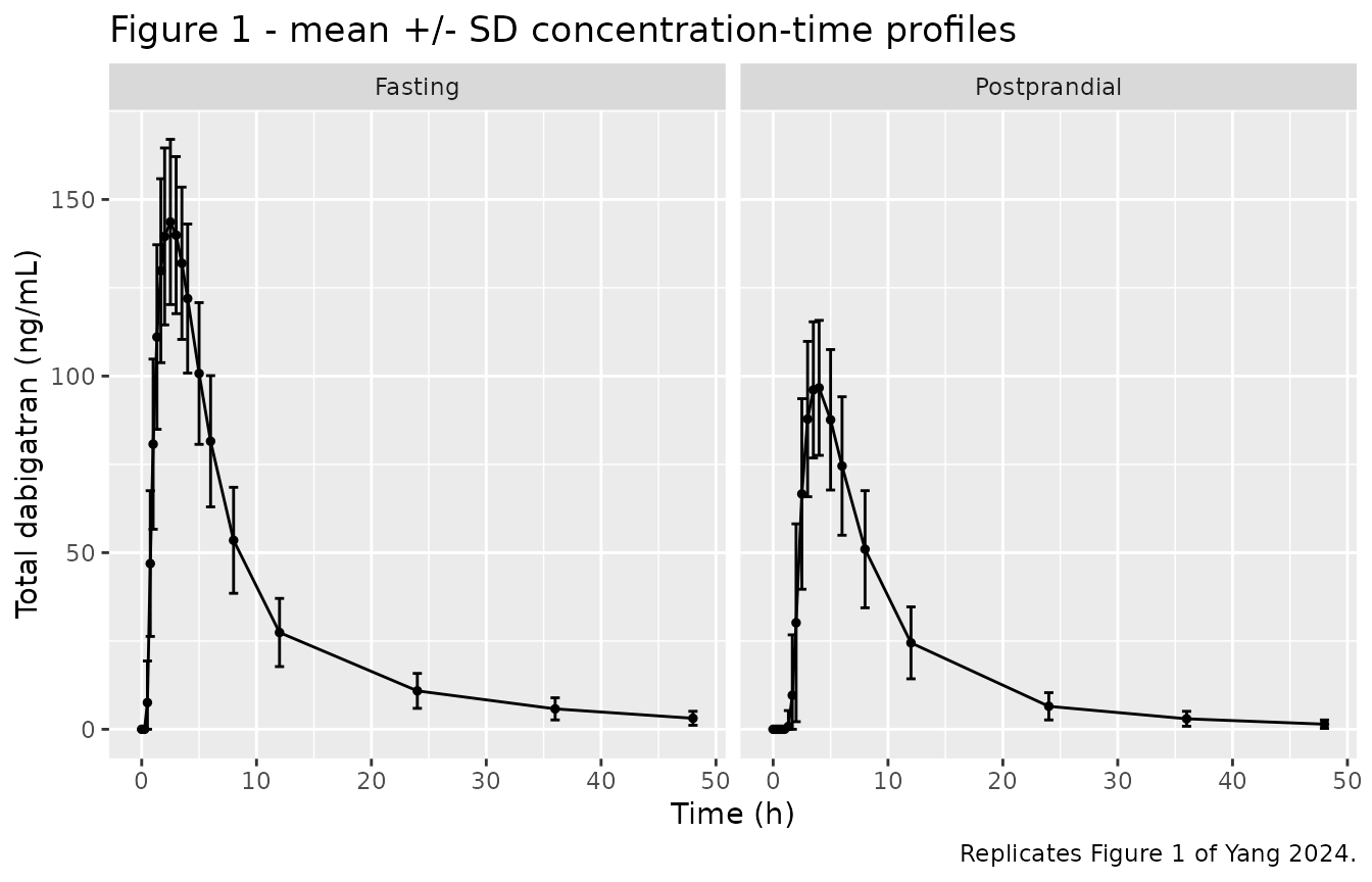
The simulated postprandial profile reproduces the two features the paper draws from Figure 1: a markedly lower peak after the high-fat meal, and a later peak.
# Replicates Figure 2 of Yang 2024 (panel a): peak (A) and 12 h trough (B)
# plasma dabigatran concentrations by ABCB1 rs4148738 genotype. Yang 2024
# Results 3.4 defines the 12 h concentration as the trough.
peaks <- sim |>
  group_by(id, genotype) |>
  summarise(Peak = max(Cc), .groups = "drop")

troughs <- sim |>
  filter(time == 12) |>
  select(id, genotype, Trough = Cc)

peaks |>
  left_join(troughs, by = c("id", "genotype")) |>
  tidyr::pivot_longer(c(Peak, Trough), names_to = "measure",
                      values_to = "conc") |>
  mutate(measure = factor(measure, levels = c("Peak", "Trough"),
                          labels = c("(A) Peak", "(B) Trough (12 h)"))) |>
  ggplot(aes(genotype, conc)) +
  geom_boxplot(outlier.size = 0.6) +
  facet_wrap(~measure, scales = "free_y") +
  labs(x = "ABCB1 rs4148738 genotype", y = "Total dabigatran (ng/mL)",
       title = "Figure 2 - peak and trough concentration by rs4148738 genotype",
       caption = "Replicates Figure 2 of Yang 2024.")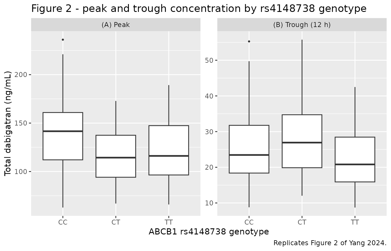
The model resolves only a CT-versus-non-CT contrast, so the CC and TT strata are structurally identical here; the paper’s own Figure 2A likewise reports no significant peak-concentration difference across genotypes, while Figure 2B singles out CT as the stratum with the lowest median trough.
PKNCA validation
sim_nca <- sim |>
  dplyr::filter(!is.na(Cc)) |>
  dplyr::select(id, time, Cc, arm, genotype)

# Guarantee a time = 0 row per subject; predose Cc = 0 for an extravascular
# single dose.
sim_nca <- dplyr::bind_rows(
  sim_nca,
  sim_nca |>
    dplyr::distinct(id, arm, genotype) |>
    dplyr::mutate(time = 0, Cc = 0)
) |>
  dplyr::distinct(id, time, .keep_all = TRUE) |>
  dplyr::arrange(id, time)

conc_obj <- PKNCA::PKNCAconc(sim_nca, Cc ~ time | arm + genotype + id)

dose_df <- events |>
  dplyr::filter(evid == 1) |>
  dplyr::select(id, time, amt, arm, genotype)

dose_obj <- PKNCA::PKNCAdose(dose_df, amt ~ time | arm + genotype + id)

intervals <- data.frame(
  start      = 0,
  end        = Inf,
  cmax       = TRUE,
  tmax       = TRUE,
  auclast    = TRUE,
  aucinf.obs = TRUE,
  half.life  = TRUE
)

nca_res <- PKNCA::pk.nca(PKNCA::PKNCAdata(conc_obj, dose_obj,
                                          intervals = intervals))
Comparison against published NCA
Yang 2024 Table 3 reports arithmetic means, so the simulated results
are aggregated with mean() rather than the median
ncaComparisonTable() would apply by default. The
food-effect rows use all 123-equivalent simulated subjects; the genotype
rows pool both meal conditions, matching the construction of Table
3.
nca_long <- as.data.frame(nca_res) |>
  dplyr::filter(PPTESTCD %in% c("cmax", "tmax", "auclast", "aucinf.obs",
                                "half.life"),
                !is.na(PPORRES))

simulated <- dplyr::bind_rows(
  nca_long |>
    dplyr::mutate(stratum = arm),
  nca_long |>
    dplyr::mutate(stratum = paste("rs4148738", genotype))
) |>
  dplyr::group_by(stratum, PPTESTCD) |>
  dplyr::summarise(PPORRES = mean(PPORRES), .groups = "drop")
# Yang 2024 Table 3, "Food effect (N = 123)" and "ABCB1 SNP rs4148738 (N = 99)"
# blocks; values are arithmetic means.
published <- tibble::tribble(
  ~stratum,             ~cmax,  ~tmax, ~auclast, ~aucinf.obs, ~half.life,
  "Fasting",            159.56, 2.39,  1352.14,  1395.65,     10.07,
  "Postprandial",       114.89, 4.44,  1049.14,  1071.37,      9.24,
  "rs4148738 CC",       149.52, 3.40,  1312.07,  1321.88,      9.10,
  "rs4148738 CT",       126.45, 3.73,  1145.77,  1192.18,      9.87,
  "rs4148738 TT",       144.10, 3.11,  1201.09,  1236.92,      9.27
)

cmp <- nlmixr2lib::ncaComparisonTable(
  simulated     = simulated,
  reference     = published,
  by            = "stratum",
  units         = c(cmax = "ng/mL", auclast = "ng*h/mL",
                    aucinf.obs = "ng*h/mL", tmax = "h", half.life = "h"),
  tolerance_pct = 20
)

knitr::kable(
  cmp,
  digits  = c(NA, NA, 1, 1, 1),
  caption = "Simulated vs. published NCA (Yang 2024 Table 3). * differs from reference by >20%."
)| NCA parameter | stratum | Reference | Simulated | % diff |
|---|---|---|---|---|
| Cmax (ng/mL) | Fasting | 160 | 146 | -8.4% |
| Cmax (ng/mL) | Postprandial | 115 | 101 | -12.4% |
| Cmax (ng/mL) | rs4148738 CC | 150 | 138 | -7.7% |
| Cmax (ng/mL) | rs4148738 CT | 126 | 116 | -8.0% |
| Cmax (ng/mL) | rs4148738 TT | 144 | 122 | -15.0% |
| Tmax (h) | Fasting | 2.39 | 2.55 | +6.8% |
| Tmax (h) | Postprandial | 4.44 | 3.77 | -15.2% |
| Tmax (h) | rs4148738 CC | 3.4 | 2.86 | -15.9% |
| Tmax (h) | rs4148738 CT | 3.73 | 3.4 | -8.9% |
| Tmax (h) | rs4148738 TT | 3.11 | 3.06 | -1.7% |
| AUC0-∞ (obs) (ng*h/mL) | Fasting | 1400 | 1330 | -4.8% |
| AUC0-∞ (obs) (ng*h/mL) | Postprandial | 1070 | 872 | -18.6% |
| AUC0-∞ (obs) (ng*h/mL) | rs4148738 CC | 1320 | 1180 | -10.8% |
| AUC0-∞ (obs) (ng*h/mL) | rs4148738 CT | 1190 | 1140 | -4.5% |
| AUC0-∞ (obs) (ng*h/mL) | rs4148738 TT | 1240 | 994 | -19.7% |
| AUClast (ng*h/mL) | Fasting | 1350 | 1270 | -6.3% |
| AUClast (ng*h/mL) | Postprandial | 1050 | 848 | -19.1% |
| AUClast (ng*h/mL) | rs4148738 CC | 1310 | 1130 | -13.8% |
| AUClast (ng*h/mL) | rs4148738 CT | 1150 | 1090 | -4.8% |
| AUClast (ng*h/mL) | rs4148738 TT | 1200 | 963 | -19.8% |
| t½ (h) | Fasting | 10.1 | 12.7 | +25.8%* |
| t½ (h) | Postprandial | 9.24 | 10.4 | +12.1% |
| t½ (h) | rs4148738 CC | 9.1 | 11.8 | +29.3%* |
| t½ (h) | rs4148738 CT | 9.87 | 11.8 | +19.5% |
| t½ (h) | rs4148738 TT | 9.27 | 11 | +18.3% |
- differs from reference by more than ±20%.
Reading the table. Every exposure row falls inside the 20% tolerance; the starred rows are all half-life.
- Fasting exposures agree well. This is the arm in which the structural parameters were reported, so it is the tightest check available: simulated AUC0-inf is 4.8% below the published mean, AUClast 6.3% below, Cmax 8.4% below, and Tmax 6.8% above. The consistent small negative bias on exposure is expected, because the published values are arithmetic means of a right-skewed distribution reported against a typical-value model.
-
Terminal half-life is over-predicted by about 20-25%, and
this is a property of the published parameters themselves. The
disposition estimates in Table 4 give an analytic terminal rate constant
of
beta = 0.0566 1/hfasting (t1/2 = 12.2 h) and0.0659 1/hpostprandial (t1/2 = 10.5 h), against the Table 3 non-compartmental means of 10.07 h and 9.24 h from the same data. PKNCA’s lambda-z on the simulated profiles returns 12.7 h and 10.4 h, i.e. it recovers the model’s own analytic half-life, so the gap is between the paper’s compartmental model and the paper’s own non-compartmental analysis, not a transcription error here. A plausible explanation is that a 48 h sampling window truncates the true terminal phase of a model whose peripheral compartment is large (V3/F = 756 L), so the WinNonlin lambda-z fit is biased short. Nothing was tuned to close the gap. -
Postprandial AUC is under-predicted by about 19%.
The published
Postprandial on CLcoefficient of 0.51 raises apparent clearance to 122 x 1.51 = 184 L/h, which implies AUC0-inf = 150 mg / 184 L/h = 814 ngh/mL, against an observed mean of 1071 ngh/mL. The discrepancy is internal to the published model: the coefficient is the least precisely estimated of the four (RSE 25.5%, 95% CI 0.26 to 0.77) and the bootstrap mean is lower still, 0.39, which would close roughly a third of the gap. - Postprandial Tmax is under-predicted by 15%. The simulated mean Tmax is 3.8 h against a published mean of 4.44 h. The published value is an arithmetic mean of individual Tmax values with a standard deviation of 2.08 h, read off a sampling grid that jumps from 4 h to 5 h, so a mean above the model’s modal Tmax is expected.
- Genotype strata. The model reproduces the ordering of Table 3 for Cmax, with CT the lowest stratum (simulated 116 ng/mL vs CC 138 and TT 122). CC and TT are structurally identical in the model (see Assumptions), so the gap between their simulated values is Monte Carlo noise: genotype is drawn independently of meal condition, so the fasting/postprandial split within each genotype stratum differs by chance from run to run.
Assumptions and deviations
-
Scale of the reported inter-individual variability. Yang 2024 Table 4 reports IIV as 0.31 (CL), 0.27 (V2) and 0.19 (ALAG) without stating whether these are variances or standard deviations, and the paper’s prose (“the interindividual variation for CL, V2, and ALAG was 12%, 8% and 10%”) quotes the parenthetical RSE column instead of the estimates. They are encoded here as omega on the standard-deviation scale, so the model’s variances are
0.31^2 = 0.0961,0.27^2 = 0.0729and0.19^2 = 0.0361.The paper’s own data settle this. For this model AUC0-inf = Dose / (CL/F) exactly, so the observed between-subject CV of AUC0-inf is an upper bound on the CL/F IIV CV. Table 3 gives AUC0-inf CVs of 33.5% (fasting) and 29.3% (postprandial), and Cmax CVs of 35.9% and 32.2%. Reading 0.31 as a standard deviation implies a CL/F IIV CV of 31.8%, which matches; reading it as a variance implies 60.3%, roughly double the observed spread and therefore incompatible with Table 3. The same comparison rules out the variance reading for V2 (27.5% vs 55.7%, against an observed Cmax CV of 35.9%).
For completeness: the Supplementary Material
$OMEGAblock holds larger numbers (0.2584, 0.4350, 0.1392), which are on the NONMEM variance scale. Those are the run’s initial estimates carried from an earlier fit, not the final estimates – the structural$THETAinitials differ from the Table 4 finals in the same way (KA 0.273 vs 0.38, CL 160.3 vs 122, V2 191.0 vs 245, ALAG1 1.056 vs 0.48) – so they do not fix the scale of Table 4. Covariate coefficients are fractions, not percentages. The Abstract and Results describe the effects as “increased ALAG and CL by 2.65% and 0.51% … decreased KA by 0.24%”. The Supplementary Material
$PKblocks write each covariate asIF(COV.EQ.1) X = ( 1 + THETA(n) ), so the tabulated values are fractional deviations. Reading them as percentages is also arithmetically impossible: a 2.65% increase in the absorption lag (0.48 to 0.49 h) cannot produce the 2.05 h postprandial Tmax delay in Table 3, whereas a 3.65-fold increase (0.48 to 1.75 h) reproduces it.-
Sign assignment of the two food-on-disposition coefficients. Table 4, the Abstract, the Results and the Discussion all assign -0.24 to KA and +0.51 to
- The Supplementary Material
$THETAinitial-estimate block carries the opposite pairing (CLYS1= -0.2359,KAYS1= +0.2276). Table 4 is used here, because it is the only source that reports final estimates, it is stated consistently in three places in the text, and it is the only reading consistent with Table 3: a high-fat meal delayed Tmax and lowered AUC, which requires a lower ka and a higher CL/F.
- The Supplementary Material
ABCB1rs4148738 reference category. The source dataset carried three genotype dummies (ABCB1C,ABCB1CT,ABCB1T) and only the CT dummy entered the final model, so the reference group is the pooled CC + TT homozygote population rather than the CC wild-type homozygote alone. The model therefore predicts identical exposures for CC and TT, which the genotype rows of the NCA comparison table reflect.Genotype distribution. Only 99 of the 123 subjects were genotyped, and the paper does not report the joint distribution of genotype and meal condition. The virtual cohort draws genotype independently of meal condition at the Table 2 marginal frequencies (CC 20/99, CT 48/99, TT 31/99).
Meal composition. The paper specifies only “a standard high-fat meal” (Methods 2.2) with no caloric or fat content, so
FED_HIGHFATis used with the register’s default semantic.Relative bioavailability. The source
$PKblock has noF1statement, so bioavailability is implicitly 1 and every clearance and volume in the model is an apparent (/F) quantity.No covariate on Q or V3, and no IIV on ka, Q or V3. This mirrors the source control stream, in which
QandV3are typical values with no random effect andKAcarries a covariate but no eta.Screened-but-unretained covariates. Age, weight, height, BMI, sex, and the other three genotyped SNPs (
ABCB1rs1045642,CES1rs2244613 and rs8192935) were tested by stepwise covariate modelling and dropped. They are recorded in the model file’scovariatesDataExcludedlist rather thancovariateData, because the paper reports no point estimates for them.No non-paper-derived parameter values. Every value in
ini()comes from Yang 2024 Table 4; the structural equations, the covariate form, the IIV form and the residual-error form come from the Supplementary Material NONMEM control stream.