Meropenem and vaborbactam (Trang 2021)
Source:vignettes/articles/Trang_2021_meropenem_vaborbactam.Rmd
Trang_2021_meropenem_vaborbactam.RmdModel and source
- Meropenem citation: Trang M, Griffith DC, Bhavnani SM, Loutit JS, Dudley MN, Ambrose PG, Rubino CM. 2021. Population pharmacokinetics of meropenem and vaborbactam based on data from noninfected subjects and infected patients. Antimicrob Agents Chemother 65:e02606-20. doi:10.1128/AAC.02606-20. Covariate-equation forms and reference values from the FDA Clinical Pharmacology review of NDA 209776 (Vabomere, 2017), section 4.2, Equations (1)-(3).
- Meropenem description: Two-compartment population PK model for intravenous meropenem (given with vaborbactam) in noninfected adults and adults with complicated urinary tract, bloodstream or other serious infections, with a sigmoidal Hill relationship between renal clearance and MDRD eGFR, a lower nonrenal clearance at eGFR <= 30 mL/min/1.73 m^2, a power effect of age on clearance, fixed allometric weight scaling, and a cumulative urine compartment for the urinary concentrations
- Vaborbactam description: Two-compartment population PK model for intravenous vaborbactam (given with meropenem) in noninfected adults and adults with complicated urinary tract, bloodstream or other serious infections, with a sigmoidal Hill relationship between renal clearance and MDRD eGFR, power effects of height on clearance and body surface area on central volume, proportional study-phase shifts on clearance and both volumes, and a cumulative urine compartment for the urinary concentrations
- Article: https://doi.org/10.1128/AAC.02606-20
- Supplement (Tables S1-S3, Figures S1-S7): supplemental file 1 of the
article (
aac.02606-20-s0001.pdf) - FDA Clinical Pharmacology review of NDA 209776 (Vabomere), section 4.2: https://www.accessdata.fda.gov/drugsatfda_docs/nda/2017/209776Orig1s000TOC.cfm
Meropenem-vaborbactam is a fixed-dose carbapenem / cyclic boronic acid beta-lactamase inhibitor combination given as 2 g + 2 g over 3 h every 8 h, with dose reductions for renal impairment. Because co-administration does not alter the PK of either drug, Trang 2021 fitted two separate population PK models, one per drug, to the same pooled phase 1 and phase 3 data set. Both are two-compartment models with zero-order infusion and first-order elimination, in which plasma and urine concentrations were co-modelled so that total clearance splits into a constant nonrenal arm and a sigmoidal Hill function of the MDRD eGFR for the renal arm:
For meropenem the covariate factors are a fixed allometric weight
term, (WT/80)^0.75, a power effect of age,
(AGE/58)^-0.526, and a 65% lower nonrenal clearance when
eGFR is at or below 30 mL/min/1.73 m^2. For vaborbactam they are a power
effect of height on CL, (HT/168)^2.24, a power effect of
body surface area on Vc, (BSA/1.88)^1.50, and proportional
shifts on CL, Vc and Vp for the phase 1 noninfected subjects relative to
the phase 3 infected patients. The paper therefore contributes two model
files, Trang_2021_meropenem and
Trang_2021_vaborbactam, documented together here.
Population
Trang 2021 pooled two phase 1 studies in noninfected adults (study
501, healthy volunteers given single and multiple ascending doses; study
504, adults with normal renal function through end-stage renal disease)
and two phase 3 studies in infected patients (study 505, TANGO I,
complicated urinary tract infection or acute pyelonephritis; study 506,
TANGO II, infections due to confirmed or suspected carbapenem-resistant
Enterobacterales). Table 1 of the paper summarises the 431
enrolled subjects: median age 53 years (18-92), weight 75.0 kg
(40.0-177), height 168 cm (145-193), BSA 1.84 m^2 (1.27-2.83), MDRD eGFR
90.1 mL/min/1.73 m^2 (4.50-338), and 55% female. The final meropenem
data set held 4,264 plasma concentrations from 91 noninfected subjects
and 322 infected patients plus 834 urine concentrations from 84
noninfected subjects; the final vaborbactam data set held 4,082 plasma
concentrations from 93 subjects and 321 patients plus 746 urine
concentrations from 75 subjects. The same information is available
programmatically via
readModelDb("Trang_2021_meropenem")()$population.
Source trace
The per-parameter origin is recorded as an in-file comment next to
each ini() entry. Parameter values are the
final models of Trang 2021 Tables 2 and 3 (the updated
models fitted after study 506 completed). The paper does not print the
covariate equations or their normalising values; those come from the FDA
review of the same analysis’ initial models (Equations 1-3 for meropenem
and the vaborbactam equations on the following page), whose parameter
values equal supplement Tables S1 and S2.
| Equation / parameter | Meropenem | Vaborbactam | Source location |
|---|---|---|---|
lcl_nonren (CL_NR, L/h) |
3.85 | 0.157 | Table 2 / Table 3 |
lcl_renal_max (CL_R,max, L/h) |
6.58 | 8.86 | Table 2 / Table 3 |
lcrcl50 (eGFR50, mL/min/1.73 m^2) |
40.0 | 49.7 | Table 2 / Table 3 |
lhill (Hill coefficient) |
1.95 | 2.25 | Table 2 / Table 3 |
lvc (Vc, L) |
17.0 | 17.1 | Table 2 / Table 3 |
lq (CLd, L/h) |
1.36 | 2.75 | Table 2 / Table 3 |
lvp (Vp, L) |
2.32 | 1.77 | Table 2 / Table 3 |
e_wt_cl, e_wt_q / e_wt_vc,
e_wt_vp
|
0.75 / 1.00 (fixed) | – | Table 2 |
e_age_cl |
-0.526 | – | Table 2 |
e_rgrp_cl_nonren |
-0.650 | – | Table 2; (1 + theta * RGRP) form, RGRP per FDA review
Eq. 1 |
e_ht_cl |
– | 2.24 | Table 3 |
e_bsa_vc |
– | 1.50 | Table 3 |
e_phase1_cl / e_phase1_vc /
e_phase1_vp
|
– | 0.517 / -0.215 / 1.28 | Table 3; (1 + theta * Phase) form per FDA review |
| IIV CL / Vc / CLd / Vp (%CV) | 44.5 / 48.4 / 51.7 / 37.7 | 45.6 / 39.4 / 34.5 / 23.0 | Table 2 / Table 3; omega^2 = log(CV^2 + 1)
|
| Plasma prop / add residual (variance) | 0.0423 / 0.0204 | 0.0372 / 0.0287 | Table 2 / Table 3 |
| Urine prop / add residual (variance) | 0.207 / 0.0511 | 0.115 / 5.46 | Table 2 / Table 3 |
| Reference WT 80 kg, AGE 58 years | yes | – | FDA review Eqs. 1-3 (initial model); Discussion (58-year-old typical patient) |
| Reference HT 168 cm, BSA 1.88 m^2; Phase = 1 for phase 1 | – | yes | FDA review vaborbactam equations |
| Hill CL-eGFR structure, two compartments | yes | yes | Results (i) and (iv); FDA review structural diagrams |
d/dt(urine) <- frac_renal * kel * central |
yes | yes | Materials and Methods: urine and plasma co-modelled to estimate CL_R and CL_NR |
Curine <- urine / (URINE_VOL_INTERVAL / 1000) |
yes | yes | urine concentrations over collection intervals (supplement Table S3) |
Typical-value checks against the paper’s own statements
The Discussion gives three typical-value numbers for meropenem: a
population mean CL of “about 10 liters/h in a 58-year-old patient with
an eGFR of 100 ml/min/1.73 m^2”, a renally cleared fraction of
“approximately 59%” at that eGFR, and a CL of “approximately 7 liters/h”
at an eGFR of 40. These follow in closed form from the model and are
checked on the solved model’s own cl and
frac_renal columns.
mod_mer <- readModelDb("Trang_2021_meropenem")
mod_vab <- readModelDb("Trang_2021_vaborbactam")

# Reference covariates of both models: 80 kg and 58 years (meropenem); 168 cm,
# BSA 1.88 m^2 and a phase 3 infected patient (vaborbactam).
ref_cov <- data.frame(
  WT = 80, AGE = 58, HT = 168, BSA = 1.88, STUDY_PHASE3 = 1,
  URINE_VOL_INTERVAL = 1000
)

# One subject, one 3-h infusion into central, plasma observation rows on the
# central state. Both models declare two endpoints (Cc, Curine), so
# observation rows carry dvid = 1 (the Cc endpoint) alongside the state name.
typical_events <- function(egfr, amt = 2000, dur = 3, times = seq(0, 24, by = 0.1), id = 1L) {
  dose <- data.frame(
    id = id, time = 0, evid = 1L, amt = amt, rate = amt / dur,
    cmt = "central", dvid = NA_integer_
  )
  obs <- data.frame(
    id = id, time = times, evid = 0L, amt = 0, rate = 0,
    cmt = "central", dvid = 1L
  )
  dplyr::bind_rows(dose, obs) |>
    dplyr::mutate(CRCL = egfr) |>
    dplyr::bind_cols(ref_cov)
}

solve_typical <- function(mod, events) {
  rxode2::rxSolve(
    mod,
    events = events, omega = NA, sigma = NA,
    returnType = "data.frame"
  )
}
chk <- dplyr::bind_rows(
  solve_typical(mod_mer, typical_events(100, times = 1)) |> dplyr::mutate(egfr = 100),
  solve_typical(mod_mer, typical_events(40, times = 1)) |> dplyr::mutate(egfr = 40)
) |>
  dplyr::select(egfr, cl, frac_renal)
#> ℹ parameter labels from comments will be replaced by 'label()'

knitr::kable(
  chk |>
    dplyr::mutate(
      published = c("CL about 10 L/h; renal fraction about 59%", "CL about 7 L/h")
    ) |>
    dplyr::rename(
      "eGFR (mL/min/1.73 m^2)" = egfr,
      "Model CL (L/h)" = cl,
      "Model renal fraction" = frac_renal,
      "Trang 2021 Discussion" = published
    ),
  digits = 3,
  caption = "Typical meropenem clearance at 58 years and the reference weight."
)| eGFR (mL/min/1.73 m^2) | Model CL (L/h) | Model renal fraction | Trang 2021 Discussion |
|---|---|---|---|
| 100 | 9.486 | 0.594 | CL about 10 L/h; renal fraction about 59% |
| 40 | 7.140 | 0.461 | CL about 7 L/h |
# Typical values: no random effects, so these are exact closed-form checks.
# A mis-transcribed CL_NR, CL_R,max, eGFR50 or Hill coefficient moves them
# outside these bands immediately.
stopifnot(
  abs(chk$cl[chk$egfr == 100] - 10) < 0.75, # 9.49 L/h: 'about 10 liters/h'
  abs(chk$frac_renal[chk$egfr == 100] - 0.59) < 0.01, # 0.594: 'approximately 59%'
  abs(chk$cl[chk$egfr == 40] - 7) < 0.5 # 7.14 L/h: 'approximately 7 liters/h'
)
Figure 2: clearance versus eGFR
Figure 2 of Trang 2021 overlays the typical-value Hill function on the individual post hoc clearances, with every covariate other than eGFR at its reference value. The typical curves are reproduced below; the step in the meropenem curve at 30 mL/min/1.73 m^2 is the lower nonrenal clearance of the renal group.
# One subject per eGFR value, solved in a single call per drug.
egfr_grid <- c(seq(5, 29.9, by = 0.1), seq(30, 340, by = 1))
grid_events <- dplyr::bind_rows(lapply(seq_along(egfr_grid), function(i) {
  typical_events(egfr_grid[i], times = 1, id = i)
}))
fig2 <- dplyr::bind_rows(
  solve_typical(mod_mer, grid_events) |> dplyr::mutate(drug = "Meropenem"),
  solve_typical(mod_vab, grid_events) |> dplyr::mutate(drug = "Vaborbactam")
) |>
  dplyr::mutate(egfr = egfr_grid[id])
#> ℹ parameter labels from comments will be replaced by 'label()'

ggplot(fig2, aes(egfr, cl)) +
  geom_line(colour = "blue") +
  facet_wrap(~drug) +
  labs(
    x = "eGFR (mL/min/1.73 m^2)", y = "Typical CL (L/h)",
    title = "Typical clearance versus eGFR",
    caption = "Replicates the model curves of Figure 2 of Trang 2021."
  )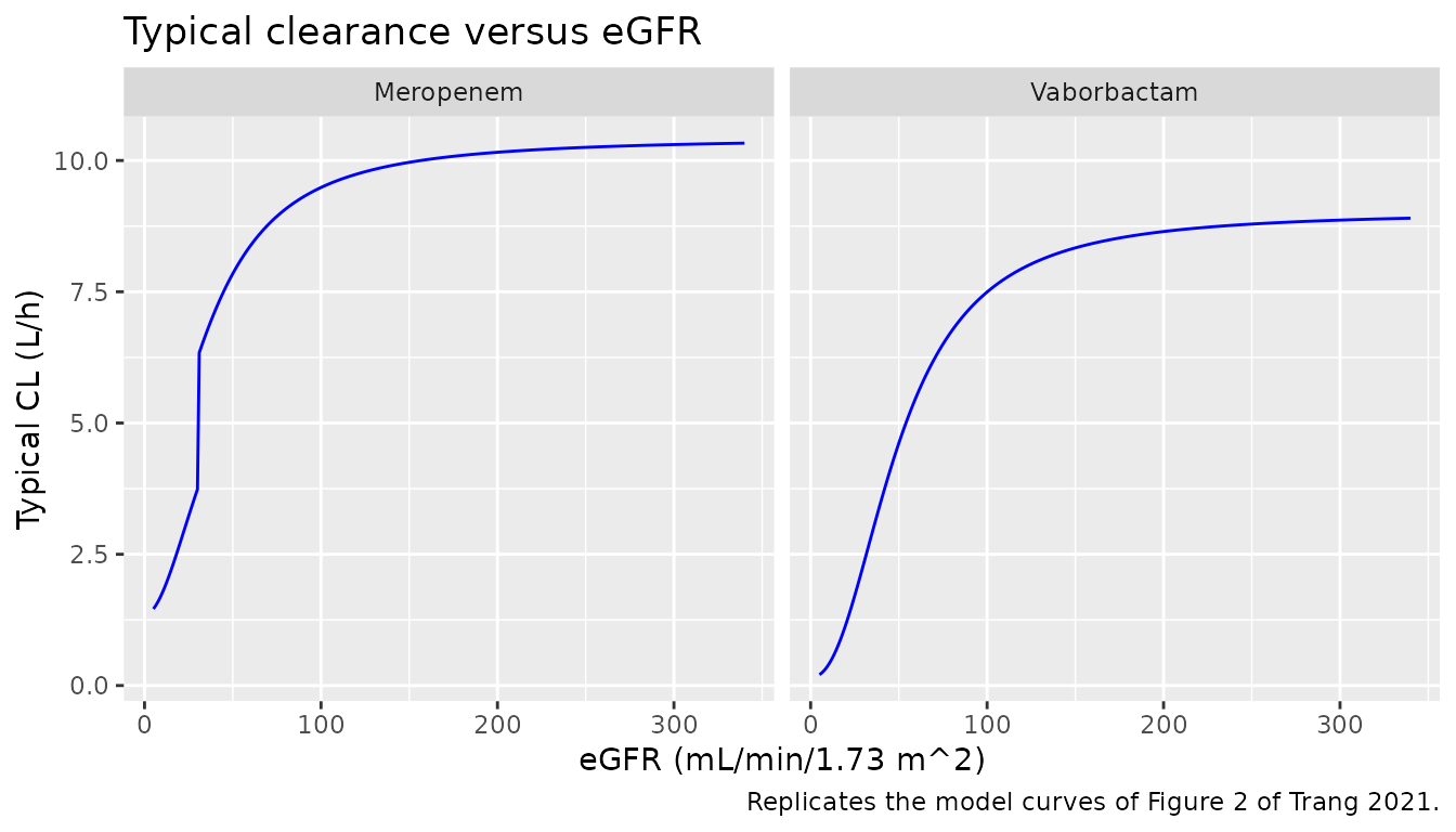
The plateau clearances are CL_NR + CL_R,max = 10.43 L/h for meropenem and 9.02 L/h for vaborbactam. The Results note that the two curves have very similar shapes, which the paper uses to argue that one eGFR-based dose adjustment serves both drugs.
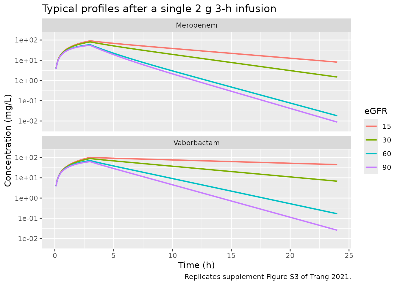
Figure S3: typical profiles by renal function
Supplement Figure S3 shows a typical infected patient given a single 2 g 3-h infusion of each drug at eGFR 15, 30, 60 and 90 mL/min/1.73 m^2. The maintainers read the 24-h concentrations off the figure’s log axis. The vaborbactam values are about 45, 7, 0.15 and 0.025 mg/L; the meropenem values at eGFR 15, 60 and 90 are about 8, 0.018 and 0.009 mg/L.
s3 <- dplyr::bind_rows(lapply(c(15, 30, 60, 90), function(e) {
  dplyr::bind_rows(
    solve_typical(mod_mer, typical_events(e)) |> dplyr::mutate(drug = "Meropenem"),
    solve_typical(mod_vab, typical_events(e)) |> dplyr::mutate(drug = "Vaborbactam")
  ) |>
    dplyr::mutate(egfr = factor(e))
}))

# Plot only (drop the pre-dose zero for the log axis); not a PKNCA input.
ggplot(s3[s3$time >= 0.1, ], aes(time, Cc, colour = egfr)) +
  geom_line(linewidth = 0.8) +
  facet_wrap(~drug, ncol = 1) +
  scale_y_log10(limits = c(0.005, 150)) +
  labs(
    x = "Time (h)", y = "Concentration (mg/L)", colour = "eGFR",
    title = "Typical profiles after a single 2 g 3-h infusion",
    caption = "Replicates supplement Figure S3 of Trang 2021."
  )
c24 <- s3 |>
  dplyr::filter(abs(time - 24) < 1e-8) |>
  dplyr::select(drug, egfr, Cc)
knitr::kable(
  c24 |> dplyr::rename("eGFR" = egfr, "Model C at 24 h (mg/L)" = Cc),
  digits = 4,
  caption = "Typical 24-h concentrations."
)| drug | eGFR | Model C at 24 h (mg/L) |
|---|---|---|
| Meropenem | 15 | 8.1486 |
| Vaborbactam | 15 | 44.9602 |
| Meropenem | 30 | 1.4898 |
| Vaborbactam | 30 | 6.8132 |
| Meropenem | 60 | 0.0181 |
| Vaborbactam | 60 | 0.1673 |
| Meropenem | 90 | 0.0088 |
| Vaborbactam | 90 | 0.0257 |
got24 <- function(d, e) c24$Cc[c24$drug == d & c24$egfr == e]
fig_read <- tibble::tribble(
  ~drug, ~egfr, ~read,
  "Vaborbactam", 15, 45,
  "Vaborbactam", 30, 7,
  "Vaborbactam", 60, 0.15,
  "Vaborbactam", 90, 0.025,
  "Meropenem", 15, 8,
  "Meropenem", 60, 0.018,
  "Meropenem", 90, 0.009
)
fig_read$model <- mapply(got24, fig_read$drug, fig_read$egfr)
# Typical values against values read off a log axis. The terminal phase spans
# four decades across the panels, so a mis-transcribed clearance or volume
# moves the 24-h value by far more than the reading error allowed here.
stopifnot(all(abs(log(fig_read$model / fig_read$read)) < log(1.5)))
All seven readings are reproduced to within a factor of 1.5. The remaining meropenem curve, eGFR = 30, is not. The model gives a 24-h concentration of 1.49 mg/L, while the figure’s green curve ends near 0.1 mg/L and its peak sits well below the eGFR-15 peak. The paper text (“an eGFR of <= 30 ml/min/1.73 m^2”) and the FDA review equation (RGRP = 1 for eGFR <= 30) both place eGFR = 30 inside the renal group. The figure is instead consistent with the full nonrenal clearance at that eGFR, as shown below with an eGFR just above the threshold. The packaged model follows the text and the equation.
Virtual phase 3 cohort
Tables 4 and 5 of Trang 2021 summarise, as geometric means, the exposures of the phase 3 patients derived from their individual post hoc parameters. The virtual cohort below approximates the Table 1 demographics of studies 505 and 506 (200 patients each). Age, height and weight are drawn around the study medians and truncated to the study ranges, BSA is computed from them by the DuBois and DuBois formula the paper used, and eGFR is drawn log-normally around the study median and truncated to the range. Doses follow the protocol renal adjustments of supplement Table S3, applied to eGFR as a stand-in for creatinine clearance. The eGFR is held constant over the simulated 5 days.
set.seed(20210817)
rxode2::rxSetSeed(20210817)

rtrunc_norm <- function(n, mean, sd, lo, hi) {
  x <- stats::rnorm(n, mean, sd)
  while (any(bad <- x < lo | x > hi)) x[bad] <- stats::rnorm(sum(bad), mean, sd)
  x
}
rtrunc_lnorm <- function(n, median, sdlog, lo, hi) {
  exp(rtrunc_norm(n, log(median), sdlog, log(lo), log(hi)))
}

# Table 1 medians and ranges per study.
study_demo <- tibble::tribble(
  ~study, ~age, ~age_lo, ~age_hi, ~ht, ~ht_lo, ~ht_hi, ~wt, ~wt_lo, ~wt_hi, ~egfr, ~egfr_lo, ~egfr_hi, ~egfr_sdlog,
  "505", 58.0, 18, 92, 165, 148, 192, 73.8, 43.8, 150, 86.9, 12.6, 241, 0.45,
  "506", 64.0, 29, 88, 168, 145, 188, 74.8, 40.0, 177, 72.1, 4.50, 338, 0.50
)

# Supplement Table S3 dose adjustment. Study 505 had only the > 50 and 30-50
# bands; the few 505 patients simulated below 30 take the 30-50 regimen.
dose_regimen <- function(study, egfr) {
  if (egfr > 50) {
    return(list(amt = 2000, ii = 8))
  }
  if (study == "505" || egfr > 30) {
    return(list(amt = 1000, ii = 8))
  }
  if (egfr > 20) {
    return(list(amt = 1000, ii = 12))
  }
  if (egfr > 10) {
    return(list(amt = 500, ii = 12))
  }
  list(amt = 500, ii = 24)
}

make_patients <- function(d, n, id_offset) {
  tibble::tibble(
    id = id_offset + seq_len(n),
    study = d$study,
    AGE = rtrunc_norm(n, d$age, 16, d$age_lo, d$age_hi),
    HT = rtrunc_norm(n, d$ht, 9, d$ht_lo, d$ht_hi),
    WT = rtrunc_lnorm(n, d$wt, 0.22, d$wt_lo, d$wt_hi),
    CRCL = rtrunc_lnorm(n, d$egfr, d$egfr_sdlog, d$egfr_lo, d$egfr_hi)
  ) |>
    dplyr::mutate(
      BSA = 0.007184 * WT^0.425 * HT^0.725,
      STUDY_PHASE3 = 1,
      URINE_VOL_INTERVAL = 1000
    )
}

patients <- dplyr::bind_rows(
  make_patients(study_demo[1, ], 200, 0L),
  make_patients(study_demo[2, ], 200, 200L)
)
patients$amt <- NA_real_
patients$ii <- NA_real_
for (i in seq_len(nrow(patients))) {
  r <- dose_regimen(patients$study[i], patients$CRCL[i])
  patients$amt[i] <- r$amt
  patients$ii[i] <- r$ii
}

obs_times <- sort(unique(c(seq(0, 24, by = 0.25), seq(96, 120, by = 0.25))))
events <- dplyr::bind_rows(lapply(seq_len(nrow(patients)), function(i) {
  p <- patients[i, ]
  dose_times <- seq(0, 120 - p$ii, by = p$ii)
  dplyr::bind_rows(
    tibble::tibble(
      id = p$id, time = dose_times, evid = 1L, amt = p$amt,
      rate = p$amt / 3, cmt = "central", dvid = NA_integer_
    ),
    tibble::tibble(
      id = p$id, time = obs_times, evid = 0L, amt = 0, rate = 0,
      cmt = "central", dvid = 1L
    )
  ) |>
    dplyr::mutate(
      study = p$study, AGE = p$AGE, HT = p$HT, WT = p$WT, BSA = p$BSA,
      CRCL = p$CRCL, STUDY_PHASE3 = 1, URINE_VOL_INTERVAL = 1000
    )
})) |>
  dplyr::arrange(id, time, dplyr::desc(evid))
stopifnot(!anyDuplicated(unique(events[, c("id", "time", "evid")])))

patients |>
  dplyr::group_by(study) |>
  dplyr::summarise(
    n = dplyr::n(),
    age = stats::median(AGE), wt = stats::median(WT), ht = stats::median(HT),
    bsa = stats::median(BSA), egfr = stats::median(CRCL),
    pct_reduced_dose = 100 * mean(amt < 2000 | ii > 8),
    .groups = "drop"
  ) |>
  dplyr::rename(
    "Study" = study, "N" = n, "Age (y)" = age, "Weight (kg)" = wt,
    "Height (cm)" = ht, "BSA (m^2)" = bsa, "eGFR" = egfr,
    "Reduced dose (%)" = pct_reduced_dose
  ) |>
knitr::kable(digits = 1, caption = "Virtual cohort medians.")| Study | N | Age (y) | Weight (kg) | Height (cm) | BSA (m^2) | eGFR | Reduced dose (%) |
|---|---|---|---|---|---|---|---|
| 505 | 200 | 58.2 | 75.7 | 164.7 | 1.8 | 86.4 | 13 |
| 506 | 200 | 63.5 | 73.0 | 167.8 | 1.8 | 72.9 | 23 |
For comparison, Table 4’s footnote records a reduced dose for 28 of 272 patients (10%) in study 505 and 9 of 50 (18%) in study 506.
Simulation
sim_mer <- rxode2::rxSolve(
  mod_mer,
  events = events, keep = c("study"), returnType = "data.frame"
) |>
  dplyr::mutate(drug = "Meropenem")
sim_vab <- rxode2::rxSolve(
  mod_vab,
  events = events, keep = c("study"), returnType = "data.frame"
) |>
  dplyr::mutate(drug = "Vaborbactam")
sim <- dplyr::bind_rows(sim_mer, sim_vab)
sim |>
  dplyr::filter(time <= 24) |>
  dplyr::group_by(drug, study, time) |>
  dplyr::summarise(
    Q05 = stats::quantile(Cc, 0.05), Q50 = stats::quantile(Cc, 0.50),
    Q95 = stats::quantile(Cc, 0.95), .groups = "drop"
  ) |>
  ggplot(aes(time, Q50)) +
  geom_ribbon(aes(ymin = Q05, ymax = Q95), alpha = 0.25) +
  geom_line() +
  facet_grid(drug ~ study) +
  scale_y_log10() +
  labs(
    x = "Time (h)", y = "Plasma concentration (mg/L)",
    title = "Simulated day-1 profiles (median and 90% interval)",
    caption = "Virtual phase 3 cohort; compare the ranges of Figure 1 of Trang 2021."
  )
#> Warning in scale_y_log10(): log-10 transformation introduced infinite values.
#> log-10 transformation introduced infinite values.
#> log-10 transformation introduced infinite values.
#> log-10 transformation introduced infinite values.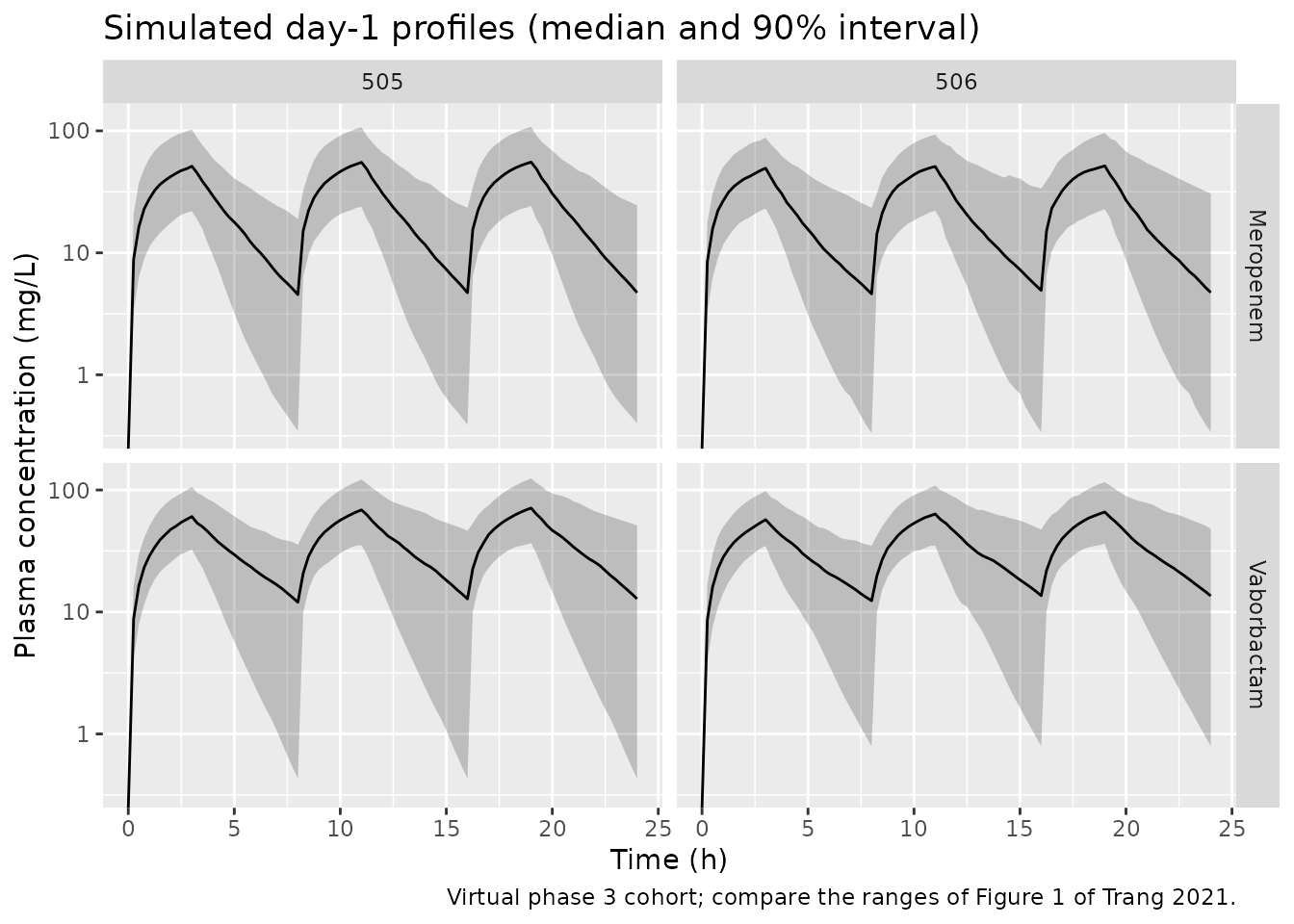
PKNCA validation
Cmax over the first dosing interval, AUC0-24 on day 1 and AUC0-24 at steady state (day 5) are computed with PKNCA per study. The paper’s exposures come from the individual post hoc parameters of the fitted patients, so the comparison is between geometric means.
nca_one <- function(sim_drug, events) {
  conc <- sim_drug |>
    dplyr::filter(!is.na(Cc)) |>
    dplyr::select(id, time, Cc, study)
  conc <- dplyr::bind_rows(
    conc,
    conc |> dplyr::distinct(id, study) |> dplyr::mutate(time = 0, Cc = 0)
  ) |>
    dplyr::distinct(id, study, time, .keep_all = TRUE) |>
    dplyr::arrange(id, time)
  doses <- events |>
    dplyr::filter(evid == 1) |>
    dplyr::select(id, time, amt, study)
  intervals <- data.frame(
    start = c(0, 0, 96), end = c(8, 24, 120),
    cmax = c(TRUE, FALSE, FALSE), auclast = c(FALSE, TRUE, TRUE)
  )
  # One PKNCA call per study keeps each call small (the cost grows faster
  # than linearly in the number of subject-intervals).
  res <- lapply(unique(conc$study), function(s) {
    cobj <- PKNCA::PKNCAconc(dplyr::filter(conc, study == s), Cc ~ time | study + id)
    dobj <- PKNCA::PKNCAdose(dplyr::filter(doses, study == s), amt ~ time | study + id)
    as.data.frame(PKNCA::pk.nca(PKNCA::PKNCAdata(cobj, dobj, intervals = intervals)))
  })
  dplyr::bind_rows(res) |>
    dplyr::filter(PPTESTCD %in% c("cmax", "auclast")) |>
    dplyr::mutate(
      window = dplyr::case_when(
        PPTESTCD == "cmax" ~ "First dose (0-8 h)",
        start == 0 ~ "Day 1 (0-24 h)",
        TRUE ~ "Steady state (96-120 h)"
      )
    )
}

nca_mer <- nca_one(sim_mer, events) |> dplyr::mutate(drug = "Meropenem")
nca_vab <- nca_one(sim_vab, events) |> dplyr::mutate(drug = "Vaborbactam")
nca_all <- dplyr::bind_rows(nca_mer, nca_vab)

geo <- function(x) exp(mean(log(x)))
sim_geo <- nca_all |>
  dplyr::group_by(drug, study, window, PPTESTCD) |>
  dplyr::summarise(PPORRES = geo(PPORRES), .groups = "drop")
Comparison against published exposures
# Trang 2021 Table 4 (meropenem) and Table 5 (vaborbactam): geometric means.
published <- tibble::tribble(
  ~drug, ~study, ~window, ~PPTESTCD, ~PPORRES,
  "Meropenem", "505", "First dose (0-8 h)", "cmax", 52.3,
  "Meropenem", "505", "Day 1 (0-24 h)", "auclast", 564,
  "Meropenem", "505", "Steady state (96-120 h)", "auclast", 548,
  "Meropenem", "506", "First dose (0-8 h)", "cmax", 75.4,
  "Meropenem", "506", "Day 1 (0-24 h)", "auclast", 802,
  "Meropenem", "506", "Steady state (96-120 h)", "auclast", 857,
  "Vaborbactam", "505", "First dose (0-8 h)", "cmax", 65.4,
  "Vaborbactam", "505", "Day 1 (0-24 h)", "auclast", 739,
  "Vaborbactam", "505", "Steady state (96-120 h)", "auclast", 710,
  "Vaborbactam", "506", "First dose (0-8 h)", "cmax", 90.4,
  "Vaborbactam", "506", "Day 1 (0-24 h)", "auclast", 1020,
  "Vaborbactam", "506", "Steady state (96-120 h)", "auclast", 1190
)

cmp <- nlmixr2lib::ncaComparisonTable(
  simulated = sim_geo,
  reference = published,
  by = c("drug", "study", "window"),
  units = c(cmax = "mg/L", auclast = "mg*h/L"),
  tolerance_pct = 20
)
knitr::kable(
  cmp,
  caption = paste(
    "Simulated vs. published geometric-mean exposures (Tables 4 and 5).",
    "* differs from the published value by more than 20%."
  )
)| NCA parameter | drug | study | window | Reference | Simulated | % diff |
|---|---|---|---|---|---|---|
| Cmax (mg/L) | Meropenem | 505 | First dose (0-8 h) | 52.3 | 51.4 | -1.8% |
| Cmax (mg/L) | Meropenem | 506 | First dose (0-8 h) | 75.4 | 47.7 | -36.7%* |
| Cmax (mg/L) | Vaborbactam | 505 | First dose (0-8 h) | 65.4 | 59.9 | -8.4% |
| Cmax (mg/L) | Vaborbactam | 506 | First dose (0-8 h) | 90.4 | 57.3 | -36.6%* |
| AUClast (mg*h/L) | Meropenem | 505 | Day 1 (0-24 h) | 564 | 614 | +8.9% |
| AUClast (mg*h/L) | Meropenem | 505 | Steady state (96-120 h) | 548 | 640 | +16.9% |
| AUClast (mg*h/L) | Meropenem | 506 | Day 1 (0-24 h) | 802 | 584 | -27.2%* |
| AUClast (mg*h/L) | Meropenem | 506 | Steady state (96-120 h) | 857 | 613 | -28.4%* |
| AUClast (mg*h/L) | Vaborbactam | 505 | Day 1 (0-24 h) | 739 | 844 | +14.2% |
| AUClast (mg*h/L) | Vaborbactam | 505 | Steady state (96-120 h) | 710 | 917 | +29.2%* |
| AUClast (mg*h/L) | Vaborbactam | 506 | Day 1 (0-24 h) | 1020 | 817 | -19.9% |
| AUClast (mg*h/L) | Vaborbactam | 506 | Steady state (96-120 h) | 1190 | 901 | -24.3%* |
# Individual CL and the alpha / beta half-lives from each subject's own
# micro-constants (the quantities Tables 4 and 5 also report).
indiv <- sim |>
  dplyr::group_by(drug, study, id) |>
  dplyr::slice(1) |>
  dplyr::ungroup() |>
  dplyr::mutate(
    a = kel + k12 + k21,
    lambda1 = (a + sqrt(a^2 - 4 * kel * k21)) / 2,
    lambda2 = (a - sqrt(a^2 - 4 * kel * k21)) / 2,
    thalf_a = log(2) / lambda1,
    thalf_b = log(2) / lambda2
  )

derived <- indiv |>
  dplyr::group_by(drug, study) |>
  dplyr::summarise(
    cl = geo(cl), thalf_a = geo(thalf_a), thalf_b = geo(thalf_b),
    .groups = "drop"
  ) |>
  dplyr::left_join(
    tibble::tribble(
      ~drug, ~study, ~cl_pub, ~thalf_a_pub, ~thalf_b_pub,
      "Meropenem", "505", 9.61, 0.751, 1.79,
      "Meropenem", "506", 4.96, 0.895, 2.61,
      "Vaborbactam", "505", 7.04, 0.377, 1.82,
      "Vaborbactam", "506", 3.15, 0.390, 3.87
    ),
    by = c("drug", "study")
  )

derived |>
  dplyr::select(drug, study, cl, cl_pub, thalf_a, thalf_a_pub, thalf_b, thalf_b_pub) |>
  dplyr::rename(
    "Drug" = drug, "Study" = study,
    "CL sim (L/h)" = cl, "CL published" = cl_pub,
    "t1/2,a sim (h)" = thalf_a, "t1/2,a published" = thalf_a_pub,
    "t1/2,b sim (h)" = thalf_b, "t1/2,b published" = thalf_b_pub
  ) |>
knitr::kable(digits = 3, caption = "Geometric means of individual CL and half-lives.")| Drug | Study | CL sim (L/h) | CL published | t1/2,a sim (h) | t1/2,a published | t1/2,b sim (h) | t1/2,b published |
|---|---|---|---|---|---|---|---|
| Meropenem | 505 | 8.554 | 9.61 | 0.743 | 0.751 | 2.181 | 1.79 |
| Meropenem | 506 | 8.205 | 4.96 | 0.733 | 0.895 | 2.239 | 2.61 |
| Vaborbactam | 505 | 5.975 | 7.04 | 0.362 | 0.377 | 2.210 | 1.82 |
| Vaborbactam | 506 | 5.576 | 3.15 | 0.393 | 0.390 | 2.377 | 3.87 |
pct_diff <- sim_geo |>
  dplyr::inner_join(published, by = c("drug", "study", "window", "PPTESTCD"),
                    suffix = c("_sim", "_pub")) |>
  dplyr::mutate(pct = 100 * (PPORRES_sim - PPORRES_pub) / PPORRES_pub)

# Study 505 is the large cUTI trial (272 of the 322 patients) whose
# demographics the virtual cohort follows most closely. Its DAY-1 geometric
# means (first-dose Cmax, day-1 AUC0-24) are the structural gate: a
# mis-transcribed CL, V or dose shifts them by tens of percent. Realised
# |% diff| on this machine: 1.8-14.2%; the Monte Carlo SE of a 200-subject
# geometric mean at ~50% CV is about 3.5%, so 25% leaves room for any cohort.
# Steady-state AUC is reported but not gated (see the text below), and study
# 506 (50 sicker patients with carbapenem-resistant infections) is reported but
# not gated.
gate <- dplyr::filter(pct_diff, study == "505", window != "Steady state (96-120 h)")
stopifnot(nrow(gate) == 4L, all(abs(gate$pct) < 25))

ss_pct <- function(d) {
  round(pct_diff$pct[pct_diff$drug == d & pct_diff$study == "505" &
    pct_diff$window == "Steady state (96-120 h)"])
}
cl_pct <- function(d) {
  x <- derived[derived$drug == d & derived$study == "505", ]
  round(100 * (x$cl - x$cl_pub) / x$cl_pub)
}
For study 505 the first-dose Cmax and day-1 AUC0-24 of both drugs fall within 25% of Tables 4 and 5. The simulated steady-state AUC0-24 runs higher: 17% for meropenem and 29% for vaborbactam. In the paper the steady-state AUC0-24 is lower than on day 1 for both drugs (548 versus 564 mg*h/L for meropenem, 710 versus 739 for vaborbactam), although a 3-h infusion every 8 h with a 2-h terminal half-life should accumulate slightly. That pattern fits the time-varying eGFR the fitted patients carried: renal function improved as their infections resolved. The virtual cohort holds eGFR at its baseline value, so its steady-state exposure keeps the day-1 clearance. Vaborbactam, cleared almost entirely by the kidney, is the more sensitive of the two. The geometric mean CLs of the study-505 cohort differ from the published values by -11% (meropenem) and -15% (vaborbactam). A gap of that size is consistent with approximating the eGFR distribution from its median and range.
Study 506 is simulated from the Table 1 medians and ranges only. Its published CL geometric means (4.96 L/h for meropenem and 3.15 L/h for vaborbactam) sit about half of the study-505 values, although the median eGFR is only 17% lower. So the 506 patients cleared both drugs more slowly than a cohort matched on median eGFR, age and body size predicts, and the simulated 506 exposures are expected to fall below the published ones. That is a limit of matching a cohort on its medians, not a defect of the model. Table 5 also excludes two 506 patients with extreme t1/2,b values of 63.5 and 50.9 h.
Urinary excretion
Both models co-fit urine concentrations collected over intervals in
the phase 1 studies. The urine state accumulates renally
excreted drug at the rate frac_renal * CL * Cc, so after a
single dose at constant eGFR its asymptote is exactly
frac_renal * dose. The check below confirms this mass
balance and then shows the interval-concentration observable,
Curine, for the 0-4, 4-8, 8-12 and 12-24 h collections of
study 501 (supplement Table S3) with a nominal collected volume.
ub <- dplyr::bind_rows(
  solve_typical(mod_mer, typical_events(117, times = c(0, 96))) |> dplyr::mutate(drug = "Meropenem"),
  solve_typical(mod_vab, typical_events(117, times = c(0, 96))) |>
    dplyr::mutate(drug = "Vaborbactam")
) |>
  dplyr::filter(time == 96) |>
  dplyr::transmute(drug, fe_96h = urine / 2000, frac_renal)
knitr::kable(ub, digits = 4, caption = "Fraction of a 2 g dose excreted in urine by 96 h at eGFR 117 (study 501 median).")| drug | fe_96h | frac_renal |
|---|---|---|
| Meropenem | 0.6034 | 0.6034 |
| Vaborbactam | 0.9801 | 0.9801 |
# Nearly all drug has left the body by 96 h, so the excreted fraction must
# equal the renal fraction of clearance to within integration error.
stopifnot(all(abs(ub$fe_96h - ub$frac_renal) < 1e-3))
# Urine collected 0-4, 4-8, 8-12 and 12-24 h after a 2 g dose. The urine state
# is reset (evid = 5, amt = 0) just after each interval end, because rxode2
# applies dose-type records before same-time observations. The volume column
# carries each interval's collected volume on the observation row.
bounds <- c(4, 8, 12, 24)
vol_ml <- c(400, 350, 300, 600)
ue <- dplyr::bind_rows(
  data.frame(
    id = 1L, time = 0, evid = 1L, amt = 2000, rate = 2000 / 3,
    cmt = "central", dvid = NA_integer_
  ),
  data.frame(
    id = 1L, time = bounds, evid = 0L, amt = 0, rate = 0,
    cmt = "central", dvid = 1L
  ),
  data.frame(
    id = 1L, time = bounds + 1e-6, evid = 5L, amt = 0, rate = 0,
    cmt = "urine", dvid = NA_integer_
  )
) |>
  dplyr::arrange(time) |>
  dplyr::mutate(
    CRCL = 117, WT = 80, AGE = 58, HT = 168, BSA = 1.88, STUDY_PHASE3 = 1,
    # Each row carries the volume of the collection interval it falls in;
    # an observation at an interval end belongs to the interval it closes.
    URINE_VOL_INTERVAL = vol_ml[pmin(pmax(findInterval(time - 1e-3, c(0, bounds)), 1L), 4L)]
  )
ur <- dplyr::bind_rows(
  solve_typical(mod_mer, ue) |> dplyr::mutate(drug = "Meropenem"),
  solve_typical(mod_vab, ue) |> dplyr::mutate(drug = "Vaborbactam")
) |>
  dplyr::filter(time %in% bounds) |>
  dplyr::transmute(
    drug,
    interval = paste0(c(0, bounds[-4]), "-", bounds, " h")[match(time, bounds)],
    amount_mg = urine, volume_ml = URINE_VOL_INTERVAL, Curine
  )
knitr::kable(ur, digits = 1, caption = "Typical urinary amounts and concentrations per collection interval.")| drug | interval | amount_mg | volume_ml | Curine |
|---|---|---|---|---|
| Meropenem | 0-4 h | 845.1 | 400 | 2112.8 |
| Meropenem | 4-8 h | 301.1 | 350 | 860.2 |
| Meropenem | 8-12 h | 48.8 | 300 | 162.7 |
| Meropenem | 12-24 h | 11.7 | 600 | 19.5 |
| Vaborbactam | 0-4 h | 1231.8 | 400 | 3079.6 |
| Vaborbactam | 4-8 h | 584.6 | 350 | 1670.3 |
| Vaborbactam | 8-12 h | 115.3 | 300 | 384.3 |
| Vaborbactam | 12-24 h | 28.3 | 600 | 47.1 |
# The interval amounts must add up to the cumulative 24-h excretion of an
# un-reset solve.
cum24 <- dplyr::bind_rows(
  solve_typical(mod_mer, typical_events(117, times = 24)) |> dplyr::mutate(drug = "Meropenem"),
  solve_typical(mod_vab, typical_events(117, times = 24)) |> dplyr::mutate(drug = "Vaborbactam")
) |>
  dplyr::filter(time == 24)
tot <- ur |>
  dplyr::group_by(drug) |>
  dplyr::summarise(sum_mg = sum(amount_mg), .groups = "drop") |>
  dplyr::left_join(dplyr::select(cum24, drug, urine), by = "drug")
stopifnot(
  all(abs(tot$sum_mg - tot$urine) < 1e-3 * tot$urine),
  all(abs(ur$Curine - ur$amount_mg / (ur$volume_ml / 1000)) < 1e-6)
)
Assumptions and deviations
-
Covariate equations and reference values. Trang
2021 prints the parameter values of the final models but not the
covariate equations or their normalising values. The functional forms
and the references (80 kg and 58 years for meropenem; 168 cm, 1.88 m^2
and the
Phaseindicator for vaborbactam) are taken from the FDA Clinical Pharmacology review of NDA 209776, which prints them for the initial models of the same analysis. The final models are refits of those models to the completed data set. The vaborbactam structure did not change (“the only modification made was fitting a full covariance matrix”). The typical profiles of supplement Figure S3 are reproduced at the FDA-review reference covariates, and the 58-year reference is the age the Discussion uses for its typical meropenem clearance. -
Meropenem reference weight. The final meropenem
model replaced the estimated weight exponents on Vc and Vp (0.487,
0.324) with fixed allometric exponents on all four parameters. The paper
does not say whether the normalising weight changed at the same time.
The maintainers kept the 80 kg of the initial model, which is the
analysis’ own documented reference. A 70 kg reference would raise
typical meropenem CL and CLd by
(80/70)^0.75, or 10%, and Vc and Vp by 14%, all at 70 kg. None of the paper’s typical-value numbers discriminates between the two, since each is stated at the reference weight. -
Renal-group shift. The initial model wrote the
renal group’s nonrenal clearance as
CL_NR * 0.349. The final Table 2 reports a “proportional shift” of -0.650. The maintainers encoded this asCL_NR * (1 - 0.650 * RGRP), the same form as the vaborbactam phase shifts. It gives a multiplier of 0.350, consistent with 0.349. RGRP is recomputed from the time-varying eGFR aseGFR <= 30. Figure S3’s eGFR-30 meropenem curve looks as if it used the full nonrenal clearance (see above). The model follows the text and the equation. -
Study phase. The source
Phaseindicator (1 = phase 1 noninfected subject) is encoded as1 - STUDY_PHASE3, so the phase 3 infected patients are the typical-value reference. The phase 1 stratum includes the renally impaired, noninfected subjects of study 504. -
Placement of the clearance IIV. Tables 2 and 3
print the clearance IIV on the
CL R,maxrow. The Results state that IIV was placed on “clearance (CL)”, and the applicant’s table reproduced in the FDA review puts it on theCLrow. The maintainers applied the eta to total clearance, as in the same group’s plazomicin model (Trang_2019_plazomicin). For vaborbactam, whose nonrenal clearance is under 2% of the total, the two readings are nearly identical. For meropenem they differ in how variable clearance is at low eGFR. -
Omitted IIV covariances. Both final models fitted a
full IIV covariance matrix, but the paper reports only the diagonal
%CVs. The etas are entered as independent, with
omega^2 = log(CV^2 + 1). - Residual-error scale. The residual-error rows of Tables 2 and 3 carry no unit label. They are read as variances (sigma^2), and the models use their square roots. Read as SDs, the plasma proportional errors would be 4.2% and 3.7%. Supplement Figures S1 and S2 rule that out: the individual weighted residuals spread across about +/-2 at concentrations of 25-75 mg/L, where the additive term is negligible, and observed values scatter about 20-30% around the individual predictions on the log observed-versus-IPRED panels. A 20% proportional SD (the variance reading) fits both. The urine residual errors are read the same way; the urine additive term is taken to be in mg/L.
-
Urine arm. The renal arm’s share of the individual
clearance (
frac_renal) is routed to theurinestate. This assumes that the weight, age, height, phase and eta factors scale renal and nonrenal clearance equally, as they do in the total-clearance equation. Urine concentrations need the collected volume of each interval (URINE_VOL_INTERVAL), and theurinestate must be reset at every interval boundary. For plasma-only simulation, any positive volume can be supplied. - Virtual cohort. Covariates are drawn independently around the Table 1 medians (no correlation between age and eGFR), and eGFR stands in for the creatinine clearance that the protocols used to adjust doses. eGFR is held constant over the simulation, although the model accepts it as time-varying.
- Errata. No correction notice for the article had been published as of 2026-09-28.